Moore's Law and Algorithms - Case of Fibonacci Numbers

The world of computers is moving fast. While going through some materials on algorithms, I have come across an interesting discussion -enhancements in hardware (cpu) vis-a-vis algorithms.

One side of the coin is the hardware - the speed of computers. The famous Moore’s law states that:

In simple words, Moore’s law is the observation that, over the history of computing hardware, the number of transistors in a dense integrated circuit has doubled approximately every two years. More precisely, the number of transistors in a dense integrated circuit has increased by a factor of 1.6 every two years. More recently, keeping up with this has been challenging. In the context of this discussion, the inherent assumption is that number of transistors is directly proportional to the speed of computers.

Now, looking at the other side of the coin - speed of algorithms. According to Excerpt from Report to the President and Congress: Designing a Digital Future, December 2010 (page 97):

The gain in computing speed due to algorithms have been simply phenomenal, unprecedented, to say the least! Being actively involved with realization of Moore’s law, I have been naturally attracted in the study and design of algorithms.

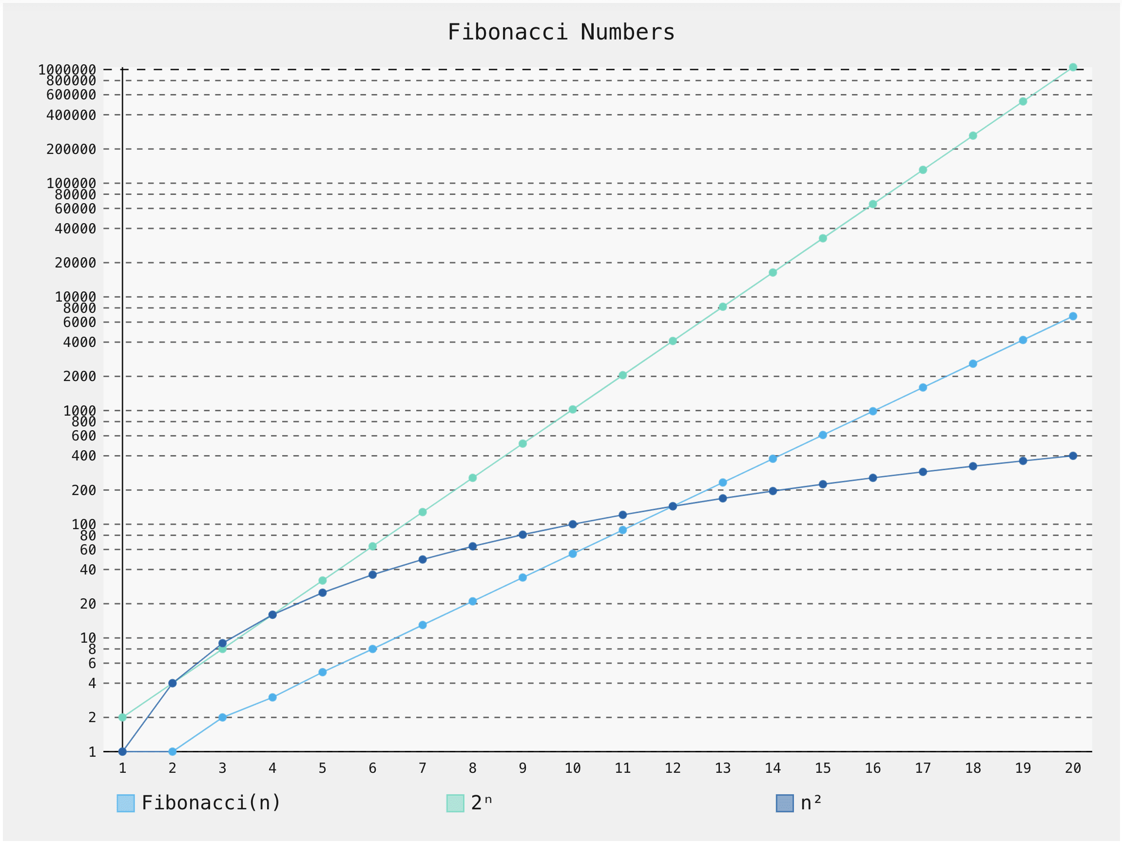
To get a more practical perspective on this, lets look at the problem of finding large Fibonacci numbers. These numbers have been used in wide areas ranging from arts to economics to biology to computer science to the game of poker! The simple definition of these numbers are:

So, first few Fibonacci numbers are: $0, 1, 1, 2, 3, 5, 8, 13, 21, 34, 55, 89, 144 \ldots$ These numbers grow almost as fast as powers of 2: for example, $F_{30}$ is over a million, and $F_{100}$ is 21 digits long! In general, $F_n \approx 2^{0.694n}$ Clearly, we need a computing device to calculate say $F_{200}$.

Here is a simple plot of first few Fibonacci numbers:

The most basic algorithm, that comes to mind is a recursive scheme that taps directly into the above definition of Fibonacci series.

def fibRecursive(n):
    if n == 0:
        return 0
    if n == 1:
        return 1
    return fibRecursive(n-2)+fibRecursive(n-1)

If you analyze this scheme, this is in fact an exponential algorithm, i.e. fibRecursive( n ) is proportional to $2^{0.694n} \approx (1.6)^n$, so it takes 1.6 times longer to compute $F_{n+1}$ than $F_n$. This is interesting. Recall, under Moore’s law, computers get roughly 1.6 times faster every 2 years. So if we can reasonably compute $F_{100}$ with this year’s technology, then only after 2 years we will manage to get $F_{101}$! Only one more Fibonacci number every 2 years!

Luckily, algorithms have grown at a much faster pace. Let’s consider improvements w.r.t to this current problem of finding $n^{th}$ Fibonacci number, $F_n$.

First problem we should realize in the above recursive scheme is that we are recalculating lower $F_n$ at each recursion level. Lets solve this issue by storing each calculation and avoiding any re-calculation!

def fibN2(n):
    a = 0
    b = 1
    if n == 0:
        return 0

    for i in range(1, n+1):
        c = a + b
        a = b
        b = c

    return b

On first glance this looks like an $\mathcal{O}(n)$ scheme, as we consider each addition as one operation. However, we should realize that as $n$ increases, addition can not be assumed as a single operation, rather every step of addition is an $\mathcal{O}(n)$ operation, recall first grade Math for adding numbers digit by digit!! Hence, this algorithm is an $\mathcal{O}(n^2)$ scheme. Can we do better?

You bet, we can! Lets consider the following scheme:

We can use a recursive scheme to calculate this matrix power using a divide and conquer scheme in $\mathcal{O}(\log{}n)$ time.

def mul(A, B):
    a, b, c = A
    d, e, f = B
    return a*d + b*e, a*e + b*f, b*e + c*f

def pow(A, n):
    if n == 1:     return A
    if n & 1 == 0: return pow(mul(A, A), n//2)
    else:          return mul(A, pow(mul(A, A), (n-1)//2))

def fibLogN(n):
    if n < 2: return n
    return pow((1,1,0), n-1)[0]

Lets think a bit harder about this. Is it really an $\mathcal{O}(\log{}n)$ scheme? It involves multiplication of numbers, the method mul(A, B). What happens when $n$ is very large? Sure, this will blow up, as typical multiplication would be an $\mathcal{O}(n^2)$ operation. So, in fact, our new scheme is $\mathcal{O}(n^2 \log{}n)$!

Luckily, we can solve even large multiplications in $\mathcal{O}(n^{log_2{3}} \approx n^{1.585})$, using Karatsuba multiplication, which is again a divide and conquer scheme.

Here is one simple implementation (Same as the above scheme, but with the following mul(A,B) method):

_CUTOFF = 1536

def mul(A, B):
    a, b, c = A
    d, e, f = B
    return multiply(a,d) + multiply(b,e), multiply(a,e) + multiply(b,f), multiply(b,e) + multiply(c,f)

def multiply(x, y):
    if x.bit_length() <= _CUTOFF or y.bit_length() <= _CUTOFF:
        return x * y

    else:
        n = max(x.bit_length(), y.bit_length())
        half = (n + 32) // 64 * 32
        mask = (1 << half) - 1
        xlow = x & mask
        ylow = y & mask
        xhigh = x >> half
        yhigh = y >> half

        a = multiply(xhigh, yhigh)
        b = multiply(xlow + xhigh, ylow + yhigh)
        c = multiply(xlow, ylow)
        d = b - a - c
        return (((a << half) + d) << half) + c

So, this final scheme is in $\mathcal{O}(n^{1.585}\log{}n)$ time.

Here is one final way of solving this problem in the same $\mathcal{O}(n^{1.585}\log{}n)$ time, but using a somewhat simpler scheme!

If we know $F_K$ and $F_{K+1}$, then we can find,

We can implement this using the Karatsuba multiplication as follows:

def fibFast(n):
    if n <= 2:
        return 1
    k = n // 2
    a = fibFast(k + 1)
    b = fibFast(k)
    if n % 2 == 1:
        return multiply(a,a) + multiply(b,b)
    else:
        return multiply(b,(2*a - b))

That’s it for today. We saw how far algorithms can go in speed for such simple problems. Let me know in the comments below, if you have any faster or alternate algorithms in mind. Have fun, May zero be with you!