A Practical Guide to Tree Based Learning Algorithms

Tree based learning algorithms are quite common in data science competitions. These algorithms empower predictive models with high accuracy, stability and ease of interpretation. Unlike linear models, they map non-linear relationships quite well. Common examples of tree based models are: decision trees, random forest, and boosted trees.

In this post, we will look at the mathematical details (along with various python examples) of decision trees, its advantages and drawbacks. We will find that they are simple and very useful for interpretation. However, they typically are not competitive with the best supervised learning approaches. In order to overcome various drawbacks of decision trees, we will look at various concepts (along with real-world examples in Python) like Bootstrap Aggregating or Bagging, and Random Forests. Another very widely used topic - Boosting will be discussed separately in a future post. Each of these approaches involves producing multiple trees that are combined to yield a single consensus prediction and often resulting in dramatic improvements in prediction accuracy.

Decision TreesSection titled Decision Trees

Decision tree is a supervised learning algorithm. It works for both categorical and continuous input (features) and output (predicted) variables. Tree-based methods partition the feature space into a set of rectangles, and then fit a simple model (like a constant) in each one. They are conceptually simple yet powerful.

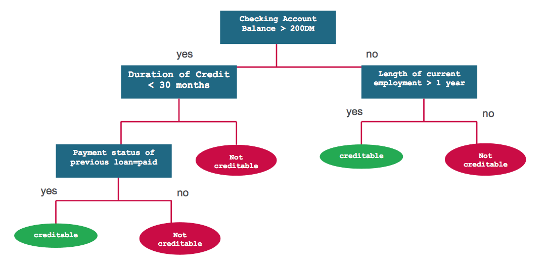
Let us first understand decision trees by an example. We will then analyze the process of building decision trees in a formal way. Consider a simple dataset of a loan lending company’s customers. We are given Checking Account Balance, Credit History, Length of Employment and Status of Previous Loan for all customers. The task is to predict the risk level of customers - creditable or not creditable. One sample solution for this problem can be depicted using the following decision tree:

Classification and Regression Trees or CART for short is a term introduced by Leo Breiman to refer to Decision Tree algorithms that can used for classification or regression predictive modeling problems. CART is one of the most common algorithms used for generating decision trees. It is used in the scikit-learn implementation of decision trees - sklearn.tree.DecisionTreeClassifier and sklearn.tree.DecisionTreeRegressor for classification and regression, respectively.

CART ModelSection titled CART Model

CART model involves selecting input variables and split points on those variables until a suitable tree is constructed. The selection of which input variable to use and the specific split or cut-point is chosen using a greedy algorithm to minimize a cost function. Tree construction ends using a predefined stopping criterion, such as a minimum number of training instances assigned to each leaf node of the tree.

Other Decision Tree AlgorithmsSection titled Other Decision Tree Algorithms

ID3 Iterative Dichotomiser 3
C4.5 successor of ID3
CHAID Chi-squared Automatic Interaction Detector
MARS: extends decision trees to handle numerical data better.
Conditional Inference Trees

Regression TreesSection titled Regression Trees

Let us look at the CART algorithm for regression trees in more detail. Briefly, building a decision tree involves two steps:

Divide the predictor space - that is, the set of possible values for $X_1, X_2, \ldots, X_p$ - into $J$ distinct and non-overlapping regions, $R_1, R_2, \ldots , R_J$ .
For every observation that falls into the region $R_j$ , make the same prediction, which is simply the mean of the response values for the training observations in $R_j$

In order to construct $J$ regions, $R_1, R_2, \ldots , R_J$ , the predictor space is divided into high-dimensional rectangles or boxes. The goal is to find boxes $R_1, R_2, \ldots , R_J$ that minimize the RSS, given by

\sum_{j=1}^{J} \sum_{i \in R_j} \big(y_i - \hat{y}_{R_j}\big)^2

where, $\hat{y}_{R_j}$ is the mean response for the training observations within the $j^{th}$ box.

Since considering every possible such partition of space is computationally infeasible, a greedy approach is used to divide the space, called recursive binary splitting. It is greedy because at each step of the tree building process, the best split is made at that particular step, rather than looking ahead and picking a split that will lead to a better tree in some future step. Note that all divided regions $R_j \forall j \in [1, J]$ would be rectangular.

In order to perform recursive binary splitting, first select the predictor $X_j$ and the cut point $s$ such that splitting the predictor space into the regions (half planes) $R_1(j,s)=\big\{ X|X_j < s \big\}$ and $R_2(j,s)=\big\{ X|X_j \ge s \big\}$ leads to the greatest possible reduction in RSS. Mathematically, we seek $j$ and $s$ that minimizes,

\sum_{i: x_i \in R_1(j,s)} \big(y_i-\hat{y}_{R_1}\big)^2 + \sum_{i: x_i \in R_2(j,s)} \big(y_i-\hat{y}_{R_2}\big)^2

where $\hat{y}_{R_1}$ is the mean response for the training observations in $R_1(j,s)$ , and $\hat{y}_{R_2}$ is the mean response for the training observations in $R_2(j,s)$ . This process is repeated, looking for the best predictor and best cut point in order to split the data further so as to minimize the RSS within each of the resulting regions. However, this time, instead of splitting the entire predictor space, only one of the two previously identified regions is split. The process continues until a stopping criterion is reached; for instance, we may continue until no region contains more than $m$ observations. Once the regions $R_1, R_2, \ldots , R_J$ have been created, the response for a given test observation is predicted using the mean of the training observations in the region to which that test observation belongs.

Classification TreesSection titled Classification Trees

A classification tree is very similar to a regression tree, except that it is used to predict a qualitative response rather than a quantitative one. Recall that for a regression tree, the predicted response for an observation is given by the mean response of the training observations that belong to the same terminal node. In contrast, for a classification tree, we predict that each observation belongs to the most commonly occurring class of training observations in the region to which it belongs (i.e. the mode response of the training observations). For the purpose of classification, many a times one is not only interested in predicting the class, rather also in probabilities of being in a given class.

The task of growing a classification tree is quite similar to the task of growing a regression tree. Just as in the regression setting, recursive binary splitting is used to grow a classification tree. However, in the classification setting, RSS cannot be used as a criterion for making the binary splits. We can replace RSS by a generic definition of node impurity measure $Q_m$ , a measure of the homogeneity of the target variable within the subset regions $R_1, R_2, \ldots , R_J$ . In a node $m$ , representing a region $R_m$ with $N_m$ observations, the proportion of training observations in the $m^{th}$ region that are from the $k^{th}$ class can be given by,

\hat{p}_{mk} = \frac{1}{N_m} \sum_{x_i \in R_m} I\big( y_i = k \big)

where, $I\big(y_i = k\big)$ is the indicator function that is 1 if $y_i = k$ , and 0 otherwise.

A natural definition of the impurity measure $Q_m$ is the classification error rate. The classification error rate is the fraction of the training observations in that region that do not belong to the most common class:

E = 1 - \max_{k}\hat{p}_{mk}

Given this is not differentiable, and hence less amenable to numerical optimization. Furthermore, this is quite insensitive to changes in the node probabilities, making classification error rate quite ineffective for growing trees. Two alternative definitions of node impurity measure that are more commonly used are gini index and cross entropy.

Gini index is a measure of total variance across the $K$ classes, defined as,

G = \sum_{k=1}^{K} \hat{p}_{mk} \big(1-\hat{p}_{mk}\big)

A small value of $G$ indicates that a node contains predominantly observations from a single class.

In information theory, Cross Entropy is a measure of degree of disorganization in a system. For a binary system, it is 0 if system contains all from the same class , and 1 if system contains equal numbers from the two classes. Hence, similar to Gini Index, Cross Entropy too can be used as a measure of node impurity, given by,

S = -\sum_{k=1}^{K} \hat{p}_{mk} \log\big(\hat{p}_{mk}\big)

Similar to $G$ , a small value of $S$ indicates that a node contains predominantly observations from a single class.

Common Parameters/ConceptsSection titled Common Parameters/Concepts

Now, that we understand decision tree mathematically, let us summarize some of the most common terms used in decision trees and tree-based learning algorithms. Understanding these terms should also be helpful in tuning models based on these methods.

Root Node Represents entire population and further gets divided into two or more sets.
Splitting Process of dividing a node into two or more sub-nodes.
Decision Node When a sub-node splits into further sub-nodes, then it is called decision node.
Leaf/ Terminal Node: Nodes that do not get split.
Branch / Sub-Tree A subsection of a tree.
Parent and Child Node A node, which is divided into sub-nodes is called parent node of sub-nodes where as sub-nodes are the child of parent node.
Minimum samples for a node split Minimum number of samples (or observations) which are required in a node to be considered for splitting. It is used to control over-fitting, higher values prevent a model from learning relations which might be highly specific to the particular sample. It should be tuned using cross validation.
Minimum samples for a terminal node (leaf) The minimum number of samples (or observations) required in a terminal node or leaf. Similar to the minimum samples for a node split, this is also used to control over-fitting. For imbalanced class problems, a lower value should be used since regions dominant with samples belonging to minority class will be much smaller in number.
Maximum depth of tree (vertical depth) The maximum depth of trees. It is used to control over-fitting, lower values prevent a model from learning relations which might be highly specific to the particular sample. It should be tuned using cross validation.
Maximum number of terminal nodes Also referred as number of leaves. Can be defined in place of max_depth. Since binary trees are created, a depth of $n$ would produce a maximum of $2^n$ leaves.
Maximum features to consider for split The number of features to consider (selected randomly) while searching for a best split. A typical value is the square root of total number of available features. A higher typically leads to over-fitting but is dependent on the problem as well.

Example of Classification TreeSection titled Example of Classification Tree

For demonstrating different tree based models, I will be using the US Income dataset available at Kaggle. You should be able to download the data from Kaggle.com. Let us first look at all the different features available in this data set.

import pandas as pd
import numpy as np
from plotnine import *
import matplotlib.pyplot as plt

from sklearn.preprocessing import LabelEncoder
from sklearn_pandas import DataFrameMapper
from sklearn.tree import DecisionTreeClassifier
from sklearn.ensemble import RandomForestClassifier

training_data = './adult-training.csv'
test_data = './adult-test.csv'

columns = ['Age','Workclass','fnlgwt','Education','EdNum','MaritalStatus',
           'Occupation','Relationship','Race','Sex','CapitalGain','CapitalLoss',
           'HoursPerWeek','Country','Income']

df_train_set = pd.read_csv(training_data, names=columns)
df_test_set = pd.read_csv(test_data, names=columns, skiprows=1)
df_train_set.drop('fnlgwt', axis=1, inplace=True)
df_test_set.drop('fnlgwt', axis=1, inplace=True)

In the above code, we imported all needed modules, loaded both test and training data as data-frames. We also got rid of the fnlgwt column that is of no importance in our modeling exercise.

Let us look at the first 5 rows of the training data:

df_train_set.head()

We also need to do some data cleanup. First, I will be removing any special characters from all columns. Furthermore, any space or ”.” characters too will be removed from any str data.

#replace the special character to "Unknown"
for i in df_train_set.columns:
    df_train_set[i].replace(' ?', 'Unknown', inplace=True)
    df_test_set[i].replace(' ?', 'Unknown', inplace=True)

for col in df_train_set.columns:
    if df_train_set[col].dtype != 'int64':
        df_train_set[col] = df_train_set[col].apply(lambda val: val.replace(" ", ""))
        df_train_set[col] = df_train_set[col].apply(lambda val: val.replace(".", ""))
        df_test_set[col] = df_test_set[col].apply(lambda val: val.replace(" ", ""))
        df_test_set[col] = df_test_set[col].apply(lambda val: val.replace(".", ""))

As you can see, there are two columns that describe education of individuals - Education and EdNum. I would assume both of these to be highly correlated and hence remove the Education column. The Country column too should not play a role in prediction of Income and hence we would remove that as well.

df_train_set.drop(["Country", "Education"], axis=1, inplace=True)
df_test_set.drop(["Country", "Education"], axis=1, inplace=True)

Although the Age and EdNum columns are numeric, they can be easily binned and be more effective. We will bin age in bins of 10 and no. of years of education into bins of 5.

colnames = list(df_train_set.columns)
colnames.remove('Age')
colnames.remove('EdNum')
colnames = ['AgeGroup', 'Education'] + colnames

labels = ["{0}-{1}".format(i, i + 9) for i in range(0, 100, 10)]
df_train_set['AgeGroup'] = pd.cut(df_train_set.Age, range(0, 101, 10), right=False, labels=labels)
df_test_set['AgeGroup'] = pd.cut(df_test_set.Age, range(0, 101, 10), right=False, labels=labels)

labels = ["{0}-{1}".format(i, i + 4) for i in range(0, 20, 5)]
df_train_set['Education'] = pd.cut(df_train_set.EdNum, range(0, 21, 5), right=False, labels=labels)
df_test_set['Education'] = pd.cut(df_test_set.EdNum, range(0, 21, 5), right=False, labels=labels)

df_train_set = df_train_set[colnames]
df_test_set = df_test_set[colnames]

Now that we have cleaned the data, let us look how balanced out data set is:

df_train_set.Income.value_counts()

# Output:

#   <=50K    24720
#   >50K      7841
#   Name: Income, dtype: int64

Similarly frequency counts for the test set are:

df_test_set.Income.value_counts()

# Output
#   <=50K    12435
#   >50K      3846
#   Name: Income, dtype: int64

In both training and the test data sets, we find $<=50K$ class to be about 3 times larger than the $>50K$ class. This is begging us to treat this problem differently as this is a problem of quite imbalanced data. However, for simplicity we will be treating this exercise as a regular problem.

EDASection titled EDA

Now, let us look at distribution and inter-dependence of different features in the training data graphically.

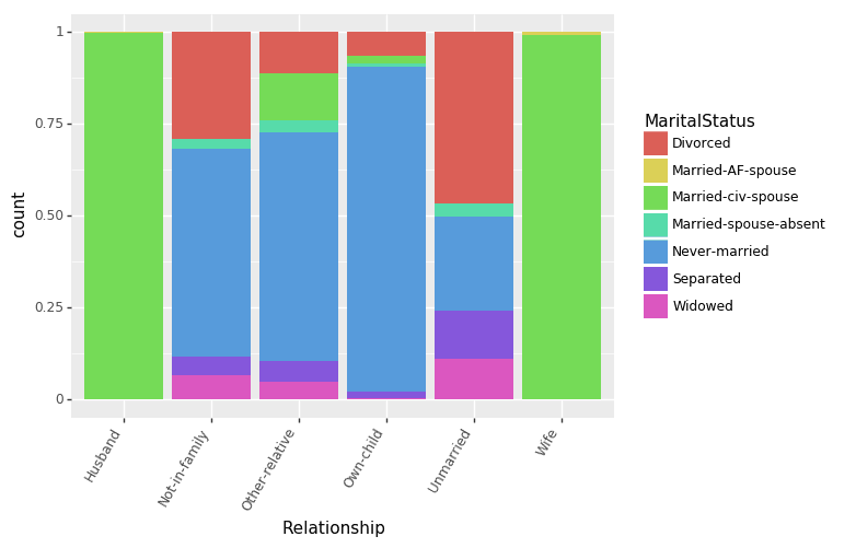
Let us first see how Relationships and MaritalStatus features are interrelated.

(ggplot(df_train_set, aes(x = "Relationship", fill = "MaritalStatus"))
 + geom_bar(position="fill")
 + theme(axis_text_x = element_text(angle = 60, hjust = 1))
)

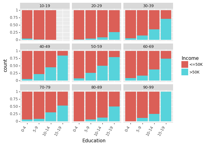
Let us look at effect of Education (measured in terms of bins of no. of years of education) on Income for different Age groups.

(ggplot(df_train_set, aes(x = "Education", fill = "Income"))
 + geom_bar(position="fill")
 + theme(axis_text_x = element_text(angle = 60, hjust = 1))
 + facet_wrap('~AgeGroup')
)

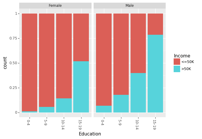
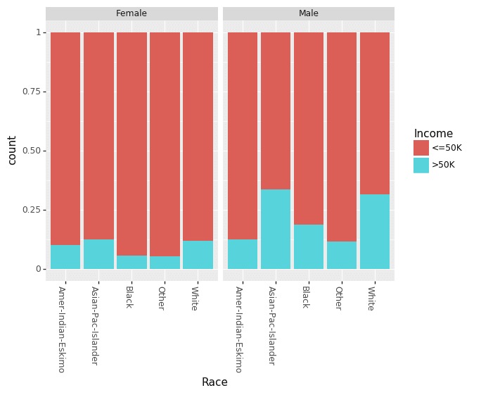
Recently, there has been a lot of talk about effect of gender based bias/gap in the income. We can look at the effect of Education and Race for males and females separately.

(ggplot(df_train_set, aes(x = "Education", fill = "Income"))
 + geom_bar(position="fill")
 + theme(axis_text_x = element_text(angle = -90, hjust = 1))
 + facet_wrap('~Sex')
)

(ggplot(df_train_set, aes(x = "Race", fill = "Income"))
 + geom_bar(position="fill")
 + theme(axis_text_x = element_text(angle = -90, hjust = 1))
 + facet_wrap('~Sex')
)

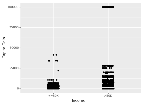
Until now, we have only looked at the inter-dependence of non-numeric features. Let us now look at the effect of CapitalGain and CapitalLoss on income.

(ggplot(df_train_set, aes(x="Income", y="CapitalGain"))
 + geom_jitter(position=position_jitter(0.1))
)

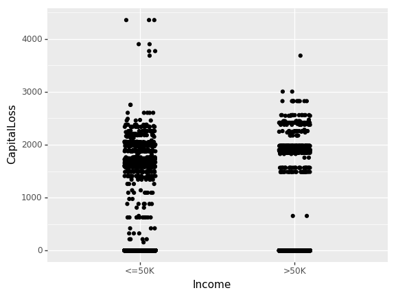
(ggplot(df_train_set, aes(x="Income", y="CapitalLoss"))
 + geom_jitter(position=position_jitter(0.1))
)

Tree Classifier

Now that we understand some relationship in our data, let us build a simple tree classifier model using sklearn.tree.DecisionTreeClassifier. However, in order to use this module, we need to convert all of our non-numeric data to numeric ones. This can be quite easily achieved using the sklearn.preprocessing.LabelEncoder module along with the sklearn_pandas module to apply this on pandas data-frames directly.

mapper = DataFrameMapper([
    ('AgeGroup', LabelEncoder()),
    ('Education', LabelEncoder()),
    ('Workclass', LabelEncoder()),
    ('MaritalStatus', LabelEncoder()),
    ('Occupation', LabelEncoder()),
    ('Relationship', LabelEncoder()),
    ('Race', LabelEncoder()),
    ('Sex', LabelEncoder()),
    ('Income', LabelEncoder())
], df_out=True, default=None)

cols = list(df_train_set.columns)
cols.remove("Income")
cols = cols[:-3] + ["Income"] + cols[-3:]

df_train = mapper.fit_transform(df_train_set.copy())
df_train.columns = cols

df_test = mapper.transform(df_test_set.copy())
df_test.columns = cols

cols.remove("Income")
x_train, y_train = df_train[cols].values, df_train["Income"].values
x_test, y_test = df_test[cols].values, df_test["Income"].values

Now we have training as well testing data in correct format to build our first model!

treeClassifier = DecisionTreeClassifier()
treeClassifier.fit(x_train, y_train)
treeClassifier.score(x_test, y_test)

The simplest possible tree classifier model with no optimization gave us an accuracy of 83.5%. In the case of classification problems, confusion matrix is a good way to judge the accuracy of models. Using the following code we can plot the confusion matrix for any of the tree-based models.

import itertools
from sklearn.metrics import confusion_matrix
def plot_confusion_matrix(cm, classes, normalize=False):
    """
    This function prints and plots the confusion matrix.
    Normalization can be applied by setting `normalize=True`.
    """
    cmap = plt.cm.Blues
    title = "Confusion Matrix"
    if normalize:
        cm = cm.astype('float') / cm.sum(axis=1)[:, np.newaxis]
        cm = np.around(cm, decimals=3)

    plt.imshow(cm, interpolation='nearest', cmap=cmap)
    plt.title(title)
    plt.colorbar()
    tick_marks = np.arange(len(classes))
    plt.xticks(tick_marks, classes, rotation=45)
    plt.yticks(tick_marks, classes)

    thresh = cm.max() / 2.
    for i, j in itertools.product(range(cm.shape[0]), range(cm.shape[1])):
        plt.text(j, i, cm[i, j],
                 horizontalalignment="center",
                 color="white" if cm[i, j] thresh else "black")

    plt.tight_layout()
    plt.ylabel('True label')
    plt.xlabel('Predicted label')

Now, we can take a look at the confusion matrix of out first model:

y_pred = treeClassifier.predict(x_test)
cfm = confusion_matrix(y_test, y_pred, labels=[0, 1])
plt.figure(figsize=(10,6))
plot_confusion_matrix(cfm, classes=["<=50K", ">50K"], normalize=True)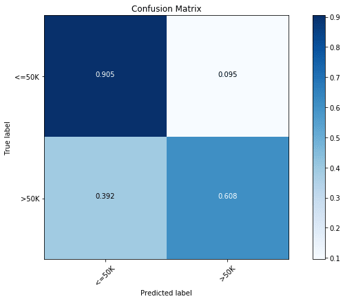

We find that the majority class ( $<=50K$ Income) has an accuracy of 90.5%, while the minority class ( $>50K$ Income) has an accuracy of only 60.8%.

Let us look at ways of tuning this simple classifier. We can use GridSearchCV() with 5-fold cross-validation to tune various important parameters of tree classifiers.

from sklearn.model_selection import GridSearchCV
parameters = {
     'max_features':(None, 9, 6),
     'max_depth':(None, 24, 16),
     'min_samples_split': (2, 4, 8),
     'min_samples_leaf': (16, 4, 12)
}

clf = GridSearchCV(treeClassifier, parameters, cv=5, n_jobs=4)
clf.fit(x_train, y_train)
clf.best_score_, clf.score(x_test, y_test), clf.best_params_

# Output
#    (0.85934092933263717,
#     0.85897672133161351,
#     {'max_depth': 16,
#      'max_features': 9,
#      'min_samples_leaf': 16,
#      'min_samples_split': 8})

With the optimization, we find the accuracy to increase to 85.9%. In the above, we can also look at the parameters of the best model. Now, let us have a look at the confusion matrix of the optimized model.

y_pred = clf.predict(x_test)
cfm = confusion_matrix(y_test, y_pred, labels=[0, 1])
plt.figure(figsize=(10,6))
plot_confusion_matrix(cfm, classes=["<=50K", ">50K"], normalize=True)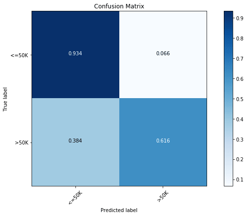

With optimization, we find an increase in the prediction accuracy of both classes.

Limitations of Decision TreesSection titled Limitations of Decision Trees

Even though decision tree models have numerous advantages,

Very simple to understand and easy to interpret
Can be visualized
Requires little data preparation. Note however that sklearn.tree module does not support missing values.
The cost of using the tree (i.e., predicting data) is logarithmic in the number of data points used to train the tree.

These models are NOT common in use directly. Some common drawbacks of decision tree are:

Can create over-complex trees that do not generalize the data well.
Can be unstable because small variations in the data might result in a completely different tree being generated.
Practical decision-tree learning algorithms are based on heuristic algorithms such as the greedy algorithm where locally optimal decisions are made at each node. Such algorithms cannot guarantee to return the globally optimal decision tree.
Decision tree learners create biased trees if some classes dominate. It is therefore recommended to balance the dataset prior to fitting with the decision tree.
Certain class of functions are difficult to model using tree models, such as XOR, parity or multiplexer.

Most of these limitations can be easily overcome by using several improvements over decision trees. In the following sections, we will be looking some of these concepts, mainly bagging, and random forests.

Tree Pruning

Since decision trees have a very high tendency to over-fit the data, a smaller tree with fewer splits (that is, fewer regions $R_1, \ldots, R_J$ ) might lead to lower variance and better interpretation at the cost of a little bias. One possible alternative to the process described above is to build the tree only so long as the decrease in the node impurity measure, $Q_m$ due to each split exceeds some (high) threshold. However, due to greedy nature of the splitting algorithm, it is too short-sighted since a seemingly worthless split early on in the tree might be followed by a very good split i.e., a split that leads to a large reduction in $Q_m$ later on.

Therefore, a better strategy is to grow a very large tree $T_0$ , and then prune it back in order to obtain a subtree. There can be several strategies to pruning, Cost complexity pruning, also known as weakest link pruning in one way to do this effectively. Rather than considering every possible subtree, a sequence of trees indexed by a non-negative tuning parameter $\alpha$ is considered. For each value of $\alpha$ there corresponds a subtree $T \subset T_0$ such that

\sum_{m=1}^{|T|}\sum_{i:x_i \in R_m}\big(y_i-\hat{y}_{R_m}\big)^2 + \alpha |T|

is as small as possible. Here $|T|$ indicates the number of terminal nodes of the tree $T$ , $R_m$ is the rectangle (i.e. the subset of predictor space) corresponding to the $m^{th}$ terminal node, and $\hat{y}_{R_m}$ is the predicted response associated with $R_m$ , i.e., the mean (or mode in the case of classification trees) of the training observations in $R_m$ .

The tuning parameter $\alpha$ controls a trade-off between the subtree’s complexity and its fit to the training data. When $\alpha = 0$ , then the subtree $T$ will simply equal $T_0$ . As $\alpha$ increases, there is a price to pay for having a tree with many terminal nodes, and so the above equation will tend to be minimized for a smaller subtree. The pruning parameter $\alpha$ can be selected using some kind of cross validation.

Note that sklearn.tree decision tree classifier (and regressor) does not currently support pruning.

Bootstrap Aggregating (Bagging)Section titled Bootstrap Aggregating (Bagging)

In statistics, bootstrapping is any test or metric that relies on random sampling with replacement. We saw above that decision trees suffer from high variance. This means that if we split the training data into two parts at random, and fit a decision tree to both halves, the results that we get could be quite different. Bootstrap aggregation, or bagging, is a general-purpose procedure for reducing the variance of a statistical learning method.

Given a set of $n$ independent observations $Z_1, Z_2, \ldots, Z_n$ , each with variance $\sigma^2$ , the variance of the mean $\bar{Z}$ of the observations is given by $\sigma^2/n$ . In other words, averaging a set of observations reduces variance. Hence a natural way to reduce the variance and hence increase the prediction accuracy of a statistical learning method is to take many training sets from the population, build a separate prediction model using each training set, and average the resulting predictions. Of there is only one problem here - we do not have access to multiple training data sets. Instead, we can bootstrap, by taking repeated samples from the (single) training data set. In this approach we generate $B$ different bootstrapped training data sets. We then train our method on the $b^{th}$ bootstrapped training set to get a prediction $\hat{f}^{*b}(x)$ to obtain one aggregate prediction,

\hat{f}_{bag} = \begin{cases} \frac{1}{B}\sum_{b=1}^{B} \hat{f}^{*b}(x) & \text{ for Regression Problems} \cr \cr \mathop{\arg\max}\limits_{b=1 \ldots B} \hat{f}^{*b}(x) & \text{ for Classification Problems} \end{cases}

This is called bagging. Note that aggregating can have different meaning in regression and classification problems. While mean prediction works well in the case of regression problems, we will need to use majority vote: the overall prediction is the most commonly occurring majority class among the B predictions, as aggregation mechanism for classification problems.

Out-of-Bag (OOB) ErrorSection titled Out-of-Bag (OOB) Error

One big advantage of bagging is that we can get testing error without any cross validation!! Recall that the key to bagging is that trees are repeatedly fit to bootstrapped subsets of the observations. One can show that on average, each bagged tree makes use of around 2/3^rd of the observations. The remaining 1/3^rd of the observations not used to fit a given bagged tree are referred to as the out-of-bag (OOB) observations. We can predict the response for the $i^{th}$ observation using each of the trees in which that observation was OOB. This will yield around $B/3$ predictions for the $i^{th}$ observation. Now using the same aggregating techniques as bagging (average for regression and majority vote for classification), we can obtain a single prediction for the $i^{th}$ observation. An OOB prediction can be obtained in this way for each of the n observations, from which the overall OOB MSE (for a regression problem) or classification error (for a classification problem) can be computed. The resulting OOB error is a valid estimate of the test error for the bagged model, since the response for each observation is predicted using only the trees that were not fit using that observation.

Feature Importance MeasuresSection titled Feature Importance Measures

Bagging typically results in improved accuracy over prediction using a single tree. However, it can be difficult to interpret the resulting model. When we bag a large number of trees, it is no longer possible to represent the resulting statistical learning procedure using a single tree, and it is no longer clear which variables are most important to the procedure. Thus, bagging improves prediction accuracy at the expense of interpret-ability.

Interestingly, one can obtain an overall summary of the importance of each predictor using the RSS (for bagging regression trees) or the Gini index (for bagging classification trees). In the case of bagging regression trees, we can record the total amount that the RSS is decreased due to splits over a given predictor, averaged over all $B$ trees. A large value indicates an important predictor. Similarly, in the context of bagging classification trees, we can add up the total amount that the Gini index is decreased by splits over a given predictor, averaged over all $B$ trees.

sklearn module’s different bagged tree-based learning methods provide direct access to feature importance data as properties once the training has finished.

Random Forest ModelsSection titled Random Forest Models

Even though bagging provides improvement over regular decision tress in terms of reduction in variance and hence improved prediction, it suffers from subtle drawbacks: Bagging requires us to make fully grown trees on bootstrapped samples, thus increasing the computational complexity by $B$ times. Furthermore, since trees in the base of bagging are correlated, the prediction accuracy will get saturated as a function of $B$ .

Random forests provide an improvement over bagged trees by way of a random small tweak that decorrelates the trees. Unlike bagging, in the case of random forests, as each tree is constructed, only a random sample of predictors is taken before each node is split. Since at the core, random forests too are bagged trees, they lead to reduction in variance. Additionally, random forests also leads to bias reduction since a very large number of predictors can be considered, and local feature predictors can play a role in the tree construction.

Random forests are able to work with a very large number of predictors, even more predictors than there are observations. An obvious gain with random forests is that more information may be brought to reduce bias of fitted values and estimated splits.

There are often a few predictors that dominate the decision tree fitting process because on the average they consistently perform just a bit better than their competitors. Consequently, many other predictors, which could be useful for very local features of the data, are rarely selected as splitting variables. With random forests computed for a large enough number of trees, each predictor will have at least several opportunities to be the predictor defining a split. In those opportunities, it will have very few competitors. Much of the time a dominant predictor will not be included. Therefore, local feature predictors will have the opportunity to define a split.

There are three main tuning parameters of random forests:

Node Size: Unlike in decision trees, the number of observations in the terminal nodes of each tree of the forest can be very small. The goal is to grow trees with as little bias as possible.
Number of Trees: In practice, few hundreds trees is often a good choice.
Number of Predictors Sampled: Typically, if there are a total of $D$ predictors, $D/3$ predictors in the case of regression and $\sqrt{D}$ predictors in the case of classification make a good choice.

Example of Random Forest ModelSection titled Example of Random Forest Model

Using the same income data as above, let us make a simple RandomForest classifier model with 500 trees.

rclf = RandomForestClassifier(n_estimators=500)
rclf.fit(x_train, y_train)
rclf.score(x_test, y_test)

Even without any optimization, we find the model to be quite close to the optimized tree classifier with a test score of 85.1%. In terms of the confusion matrix, we again find this to be quite comparable to the optimized tree classifier with a prediction accuracy of 92.1% for the majority class ( $<=50K$ Income) and a prediction accuracy of 62.6% for the minority class ( $>50K$ Income).

y_pred = rclf.predict(x_test)
cfm = confusion_matrix(y_test, y_pred, labels=[0, 1])
plt.figure(figsize=(10,6))
plot_confusion_matrix(cfm, classes=["<=50K", ">50K"], normalize=True)

As discussed before, random forest models also provide us with a metric of feature importance. We can see importance of different features in our current model as below:

importances = rclf.feature_importances_
indices = np.argsort(importances)
cols = [cols[x] for x in indices]
plt.figure(figsize=(10,6))
plt.title('Feature Importances')
plt.barh(range(len(indices)), importances[indices], color='b', align='center')
plt.yticks(range(len(indices)), cols)
plt.xlabel('Relative Importance')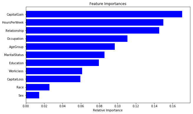

Now, let us try to optimize our random forest model. Again, this can be done using the GridSearchCV() apt with 5-fold cross-validation as below:

parameters = {
     'n_estimators':(100, 500, 1000),
     'max_depth':(None, 24, 16),
     'min_samples_split': (2, 4, 8),
     'min_samples_leaf': (16, 4, 12)
}

clf = GridSearchCV(RandomForestClassifier(), parameters, cv=5, n_jobs=8)
clf.fit(x_train, y_train)
clf.best_score_, clf.best_params_

# [OUTPUT]:
#     0.86606676699118579
#     {'max_depth': 24,
#      'min_samples_leaf': 4,
#      'min_samples_split': 4,
#      'n_estimators': 1000}

We can see this model to be significantly better than our all previous models, with a prediction rate of 86.6%. In terms of confusion matrix though, we see a significant increase in the prediction accuracy of the majority class ( $<= 50K$ Income) with slight decrease in the accuracy for the minority class ( $>50K$ Income). This is a common problem with classification problems with imbalanced data.

rclf2 = RandomForestClassifier(n_estimators=1000,max_depth=24,min_samples_leaf=4,min_samples_split=8)
rclf2.fit(x_train, y_train)

y_pred = rclf2.predict(x_test)
cfm = confusion_matrix(y_test, y_pred, labels=[0, 1])
plt.figure(figsize=(10,6))
plot_confusion_matrix(cfm, classes=["<=50K", ">50K"], normalize=True)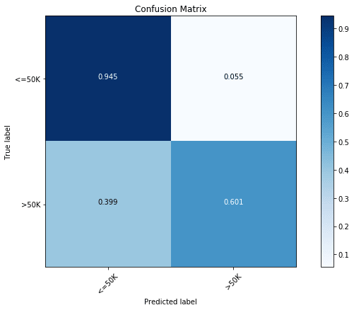

Finally, let us also look at the feature importance from the best model.

importances = rclf2.feature_importances_
indices = np.argsort(importances)
cols = [cols[x] for x in indices]
plt.figure(figsize=(10,6))
plt.title('Feature Importances')
plt.barh(range(len(indices)), importances[indices], color='b', align='center')
plt.yticks(range(len(indices)), cols)
plt.xlabel('Relative Importance')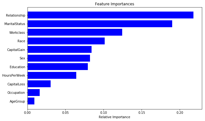

We can see the answer to be significantly different than the previous random forest model. This is a common issue with this class of models! In the next post, I will be talking about boosted tree that provide a significant improvement in terms of model consistency.

Limitations of Random ForestsSection titled Limitations of Random Forests

Apart from generic limitations of bagged trees, some of limitations of random forests are:

Random forests don’t do well at all when you require extrapolation outside of the range of the dependent (or independent) variables - better to use other algorithms like e.g., MARS
They are quite slow at both training and prediction.
They don’t deal well with a large number of categories in categorical variables.

Overall, Random Forest is usually less accurate than Boosting on a wide range of tasks, and usually slower in the runtime. In the next post, we will look at the details of boosting. I hope this post has helped you understand tree based methods in more detail now. Please let me know what topics I missed or should have been more clear about. You can also let me know in the comments below if there is any particular algorithm/topic that you want me to write about!

Machine Learning, Algorithms