A Practical guide to Autoencoders using Keras

Usually in a conventional neural network, one tries to predict a target vector y from input vectors x. In an auto-encoder network, one tries to predict x from x. It is trivial to learn a mapping from x to x if the network has no constraints, but if the network is constrained the learning process becomes more interesting.

In this article, we are going to take a detailed look at the mathematics of different types of autoencoders (with different constraints) along with a sample implementation of it using Keras, with a tensorflow back-end.

Please not that this post has been written using Tensorflow 1.x version of Keras

Table of ContentsSection titled Table of Contents

Open Table of Contents

Basic Autoencoders
Autoencoders in Practice
Sparsity Constraint
Deep Autoencoders
Convolutional Autoencoders
Denoising Autoencoders
Variational Autoencoders (VAE)
Usage of Autoencoders

Basic AutoencodersSection titled Basic Autoencoders

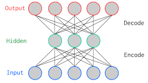
The simplest AutoEncoder (AE) has an MLP-like (Multi Layer Perceptron) structure:

Input Layer
Hidden Layer, and
Output Layer

However, unlike MLP, autoencoders do not require any target data. As the network is trying to learn $x$ itself, the learning algorithm is a special case of unsupervised learning.

A Typical Autoencoder Network

Mathematically, lets define:

Input vector: $x \in \Big[ 0, 1 \Big]^d$
Activation function: $a(h)$ applied to very nuron of layer $h$
$W_i \in \mathbb{R}^{I_{di} \times O_{di}}$ , the parameter matrix of $i$ -th layer, projecting a $I_{di}$ dimensional input in a $O_{di}$ dimensional space
$b_i \in \mathbb{R}^{O_{di}}$ bias vector

The simplest AE can then be summarized as:

\begin{aligned} z &= a(x W_1 + b_1) \cr x' &= a(z W_2 + b_2) \end{aligned}

The AE model tries to minimize the reconstruction error between the input value $x$ and the reconstructed value $x'$ . A typical definition of the reconstruction error is the $L_p$ distance (like $L_2$ norm) between the $x$ and $x'$ vectors:

\min \mathcal{L} = \min E(x, x') \stackrel{e.g.}{=} \min || x - x' ||_p

Another common variant of loss function (especially images) for AE is the cross entropy function.

\mathcal{L}(x, x') = -\sum_{c=1}^{M} x'_c \log (x_c)

where $M$ is the dimensionality of the input data $x$ (for eg. no. of pixels in an image).

Autoencoders in PracticeSection titled Autoencoders in Practice

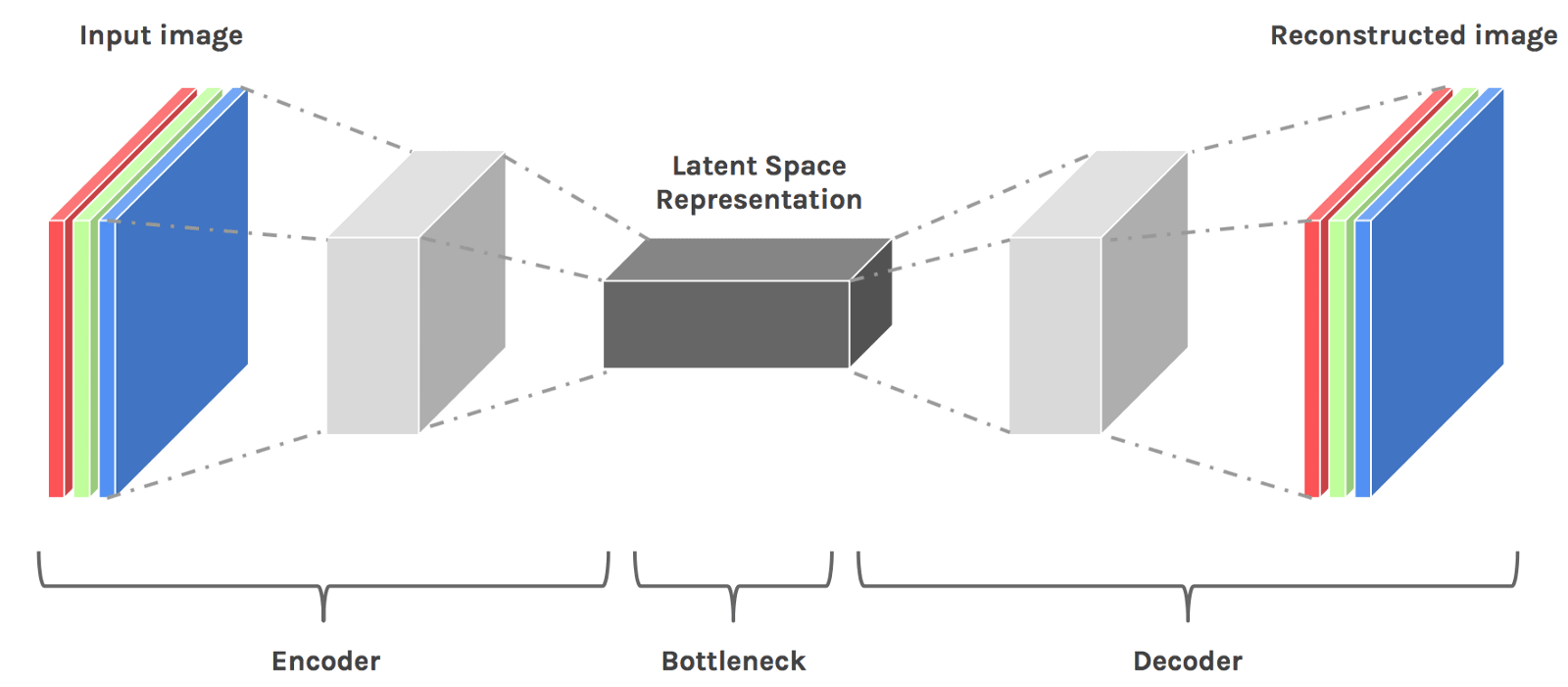
The above example of auto-encoder is too simplistic for any real use case. It can be easily noticed that if the number of units in the hidden layer is greater than or equal to the number of input units, the network will learn the identity function easily. Hence, the simplest constraint used in real-life autoencoders is the number of hidden units ( $z$ ) should be less than the dimensions ( $d$ ) of the input ( $z < d$ ).

By limiting the amount of information that can flow through the network, AE model can learn the most important attributes of the input data and how to best reconstruct the original input from an “encoded” state. Ideally, this encoding will learn and describe latent attributes of the input data. Dimensionality reduction using AEs leads to better results than classical dimensionality reduction techniques such as PCA due to the non-linearity and the type of constraints applied.

PCA and Autoencoders

If we were to construct a linear network (i.e. without the use of nonlinear activation functions at each layer) we would observe a similar dimensionality reduction as observed in PCA. See Geoffrey Hinton’s discussion.

A practical auto-encoder network consists of an encoding function (encoder), and a decoding function (decoder). Following is an example architecture for the reconstruction of images.

In this article we will build different types of autoencoders for the fashion MNIST dataset. In stead of using more common MNIST dataset, I prefer to use fashion MNIST dataset for the reasons described here.

For example using MNIST data, please have a look at the article by Francois Chollet, the creator of Keras. The code below is heavily adapted from his article.

We’ll start simple, with a single fully-connected neural layer as encoder and as decoder.

from keras.layers import Input, Dense
from keras.models import Model
import numpy as np

# size of bottleneck latent space
encoding_dim = 32
# input placeholder
input_img = Input(shape=(784,))
# encoded representation
encoded = Dense(encoding_dim, activation='relu')(input_img)
# lossy reconstruction
decoded = Dense(784, activation='sigmoid')(encoded)

# full AE model: map an input to its reconstruction
autoencoder = Model(input_img, decoded)

We will also create separate encoding and decoding functions, that can be used to extract latent features at test time.

# encoder: map an input to its encoded representation
encoder = Model(input_img, encoded)
# placeholder for an encoded input
encoded_input = Input(shape=(encoding_dim,))
# last layer of the autoencoder model
decoder_layer = autoencoder.layers[-1]
# decoder
decoder = Model(encoded_input, decoder_layer(encoded_input))

We can now set the optimizer and the loss function before training the auto-encoder model.

autoencoder.compile(optimizer='rmsprop', loss='binary_crossentropy')

Next, we need to get the [fashion MNIST] data and normalize it for training. Furthermore, we will flatten the $28\times28$ images to a vector of size 784. Please note that running the code below for the first time will download the full dataset and hence might take few minutes.

from keras.datasets import fashion_mnist

(x_train, _), (x_test, _) = fashion_mnist.load_data()
x_train = x_train.astype('float32') / 255.
x_test = x_test.astype('float32') / 255.
x_train = x_train.reshape((len(x_train), np.prod(x_train.shape[1:])))
x_test = x_test.reshape((len(x_test), np.prod(x_test.shape[1:])))
print(x_train.shape, x_test.shape)

# Output:
    (60000, 784) (10000, 784)

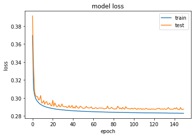
# We can now train our model for 100 epochs:

history = autoencoder.fit(x_train, x_train,
                epochs=100,
                batch_size=256,
                shuffle=True,
                validation_data=(x_test, x_test))

This will print per epoch training and validation loss. But we can plot the loss history during training using the history object.

import matplotlib.pyplot as plt

def plot_train_history_loss(history):
    # summarize history for loss
    plt.plot(history.history['loss'])
    plt.plot(history.history['val_loss'])
    plt.title('model loss')
    plt.ylabel('loss')
    plt.xlabel('epoch')
    plt.legend(['train', 'test'], loc='upper right')
    plt.show()

plot_train_history_loss(history)

Output:

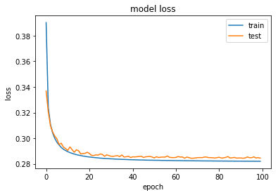
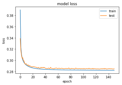
After 100 epochs, the auto-encoder reaches a stable train/text loss value of about 0.282. Let us look visually how good of reconstruction this simple model does!

# encode and decode some images from test set
encoded_imgs = encoder.predict(x_test)
decoded_imgs = decoder.predict(encoded_imgs)

def display_reconstructed(x_test, decoded_imgs, n=10):
    plt.figure(figsize=(20, 4))
    for i in range(n):
        # display original
        ax = plt.subplot(2, n, i + 1)
        plt.imshow(x_test[i].reshape(28, 28))
        plt.gray()
        ax.get_xaxis().set_visible(False)
        ax.get_yaxis().set_visible(False)

        if decoded_imgs is not None:
            # display reconstruction
            ax = plt.subplot(2, n, i + 1 + n)
            plt.imshow(decoded_imgs[i].reshape(28, 28))
            plt.gray()
            ax.get_xaxis().set_visible(False)
            ax.get_yaxis().set_visible(False)
    plt.show()

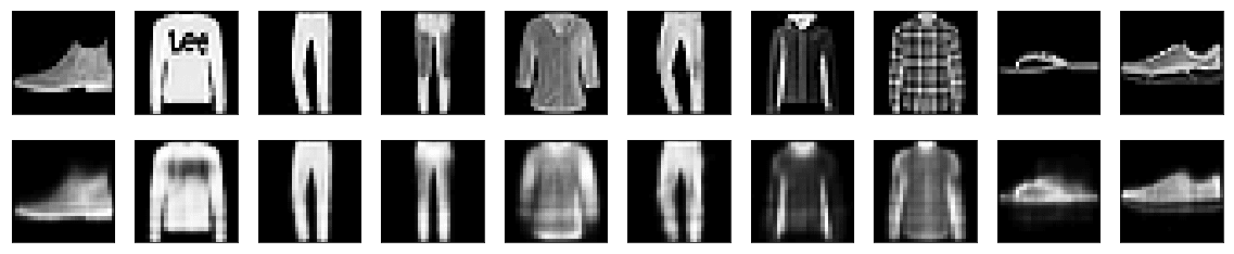
display_reconstructed(x_test, decoded_imgs, 10)

The top row is the original image, while bottom row is the reconstructed image. We can see that we are loosing a lot of fine details.

Sparsity ConstraintSection titled Sparsity Constraint

We can add an additional constraint to the above AE model, a sparsity constraints on the latent variables. Mathematically, this is achieved by adding a sparsity penalty $\Omega(\mathbf{h})$ on the bottleneck layer $\mathbf{h}$ .

\min \mathcal{L} = \min E(x, x') + \Omega(h)

where, $\mathbf{h}$ is the encoder output.

Sparsity is a desired characteristic for an auto-encoder, because it allows to use a greater number of hidden units (even more than the input ones) and therefore gives the network the ability of learning different connections and extract different features (w.r.t. the features extracted with the only constraint on the number of hidden units). Moreover, sparsity can be used together with the constraint on the number of hidden units: an optimization process of the combination of these hyper-parameters is required to achieve better performance.

In Keras, sparsity constraint can be achieved by adding an activity_regularizer to our Dense layer:

from keras import regularizers

encoding_dim = 32

input_img = Input(shape=(784,))
# add a Dense layer with a L1 activity regularizer
encoded = Dense(encoding_dim, activation='relu',
                activity_regularizer=regularizers.l1(1e-8))(input_img)
decoded = Dense(784, activation='sigmoid')(encoded)

autoencoder = Model(input_img, decoded)

Similar to the previous model, we can train this as well for 150 epochs. Using a regularizer is less likely to overfit and hence can be trained for longer.

autoencoder.compile(optimizer='rmsprop', loss='binary_crossentropy')
history = autoencoder.fit(x_train, x_train,
                epochs=150,
                batch_size=256,
                shuffle=True,
                validation_data=(x_test, x_test))

plot_train_history_loss(history)

We get a very similar loss as the previous example. Here is a plot of loss values during training.

As expected, the reconstructed images too look quite similar as before.

decoded_imgs = autoencoder.predict(x_test)
display_reconstructed(x_test, decoded_imgs, 10)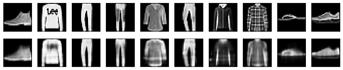

Deep AutoencodersSection titled Deep Autoencoders

We have been using only single layers for encoders and decoders. Given we have large enough data, there is nothing that stops us from building deeper networks for encoders and decoders.

input_img = Input(shape=(784,))
encoded = Dense(128, activation='relu')(input_img)
encoded = Dense(64, activation='relu')(encoded)
encoded = Dense(32, activation='relu')(encoded)

decoded = Dense(64, activation='relu')(encoded)
decoded = Dense(128, activation='relu')(decoded)
decoded = Dense(784, activation='sigmoid')(decoded)

autoencoder = Model(input_img, decoded)

We can train this model, same as before.

autoencoder.compile(optimizer='rmsprop', loss='binary_crossentropy')
history = autoencoder.fit(x_train, x_train,
                epochs=150,
                batch_size=256,
                shuffle=True,
                validation_data=(x_test, x_test))

plot_train_history_loss(history)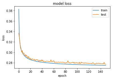

The average loss is now 0.277, as compared to ~0.285 before! We can also see that visually all reconstructed images too look slightly better.

decoded_imgs = autoencoder.predict(x_test)
display_reconstructed(x_test, decoded_imgs, 10)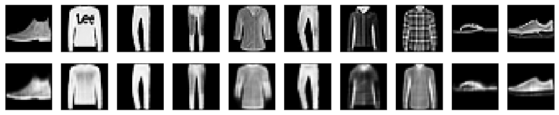

Convolutional AutoencodersSection titled Convolutional Autoencoders

Since our inputs are images, it makes sense to use convolution neural networks (conv-nets) as encoders and decoders. In practical settings, autoencoders applied to images are always convolution autoencoders —they simply perform much better.

The encoder will consist of a stack of Conv2D and MaxPooling2D layers (max pooling being used for spatial down-sampling), while the decoder will consist of a stack of Conv2D and UpSampling2D layers. We will also be using BatchNormalization. One major difference between this network and prior ones is that now we have 256 (4x4x16) elements in the bottleneck layer as opposed to just 32 before!

You can read more about convolution-based auto-encoders in further details here.

from keras.layers import Input, Dense, Conv2D, MaxPooling2D, UpSampling2D, BatchNormalization
from keras.models import Model
from keras import backend as K

input_img = Input(shape=(28, 28, 1))

x = Conv2D(32, (3, 3), activation='relu', padding='same', use_bias=False)(input_img)
x = BatchNormalization(axis=-1)(x)
x = MaxPooling2D((2, 2), padding='same')(x)
x = Conv2D(16, (3, 3), activation='relu', padding='same', use_bias=False)(x)
x = BatchNormalization(axis=-1)(x)
x = MaxPooling2D((2, 2), padding='same')(x)
x = Conv2D(16, (3, 3), activation='relu', padding='same', use_bias=False)(x)
x = BatchNormalization(axis=-1)(x)
encoded = MaxPooling2D((2, 2), padding='same')(x)

x = Conv2D(16, (3, 3), activation='relu', padding='same', use_bias=False)(encoded)
x = BatchNormalization(axis=-1)(x)
x = UpSampling2D((2, 2))(x)
x = Conv2D(16, (3, 3), activation='relu', padding='same', use_bias=False)(x)
x = BatchNormalization(axis=-1)(x)
x = UpSampling2D((2, 2))(x)
x = Conv2D(32, (3, 3), activation='relu', padding='valid', use_bias=False)(x)
x = BatchNormalization(axis=-1)(x)
x = UpSampling2D((2, 2))(x)
decoded = Conv2D(1, (3, 3), activation='sigmoid', padding='same', use_bias=False)(x)

autoencoder = Model(input_img, decoded)
autoencoder.compile(optimizer='rmsprop', loss='binary_crossentropy')

To train it, we will use the original fashion MNIST digits with shape (samples, 1, 28, 28), and we will just normalize pixel values between 0 and 1.

(x_train, _), (x_test, _) = fashion_mnist.load_data()

x_train = x_train.astype('float32') / 255.
x_test = x_test.astype('float32') / 255.
x_train = np.reshape(x_train, (len(x_train), 28, 28, 1))
x_test = np.reshape(x_test, (len(x_test), 28, 28, 1))

Similar to before, we can train this model for 150 epochs. However, unlike before, we will checkpoint the model during training to save the best model, based on the validation loss minima.

from keras.callbacks import ModelCheckpoint

fpath = "weights-ae-{epoch:02d}-{val_loss:.3f}.hdf5"
callbacks = [ModelCheckpoint(fpath, monitor='val_loss', verbose=1, save_best_only=True, mode='min')]
history = autoencoder.fit(x_train, x_train,
                epochs=150,
                batch_size=256,
                shuffle=True,
                validation_data=(x_test, x_test),
                callbacks=callbacks)

plot_train_history_loss(history)

We find the lowest validation loss now is 0.265, significantly lower than the previous best value of 0.277. We will first load the saved best model weights, and then plot the original and the reconstructed images from the test dataset.

autoencoder.load_weights('weights-ae-146-0.266.hdf5')
decoded_imgs = autoencoder.predict(x_test)
display_reconstructed(x_test, decoded_imgs, 10)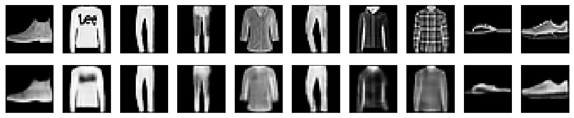

At first glance, it seems not much of improvement over the deep autoencoders result. However, if you notice closely, we start to see small feature details to appear on the reconstructed images. In order to improve these models further, we will likely have to go for deeper and more complex convolution network.

Denoising AutoencodersSection titled Denoising Autoencoders

Another common variant of AE networks is the one that learns to remove noise from the input. Mathematically, this is achieved by modifying the reconstruction error of the loss function.

Traditionally, autoencoders minimize some loss function:

L\Big(x, g\big(f(x)\big)\Big)

where, $L$ is a loss function penalizing reconstructed input $g\big(f(x)\big)$ for being dissimilar to the input $x$ . Also, $g(.)$ is the decoder and $f(.)$ is the encoder. A Denoising autoencoders (DAE) instead minimizes,

L\Big(x, g\big(f(\hat{x})\big)\Big)

where, $\hat{x}$ is a copy of $x$ that has been corrupted by some form of noise. DAEs must therefore undo this corruption rather than simply copying their input. Training of DAEs forces $f(.)$ , the encoder and $g(.)$ , the decoder to implicitly learn the structure of $p_{data}(x),$ the distribution of the input data $x$ . Please refer to the works of Alain and Bengio (2013) and Bengio et al. (2013).

For a example, we will first introduce noise to our train and test data by applying a guassian noise matrix and clipping the images between 0 and 1.

(x_train, _), (x_test, _) = fashion_mnist.load_data()

x_train = x_train.astype('float32') / 255.
x_test = x_test.astype('float32') / 255.
x_train = np.reshape(x_train, (len(x_train), 28, 28, 1))
x_test = np.reshape(x_test, (len(x_test), 28, 28, 1))

noise_factor = 0.5
x_train_noisy = x_train + noise_factor * np.random.normal(loc=0.0, scale=1.0, size=x_train.shape)
x_test_noisy = x_test + noise_factor * np.random.normal(loc=0.0, scale=1.0, size=x_test.shape)

x_train_noisy = np.clip(x_train_noisy, 0., 1.)
x_test_noisy = np.clip(x_test_noisy, 0., 1.)

Here is how the corrupted images look now. They are barely recognizable now!

display_reconstructed(x_test_noisy, None)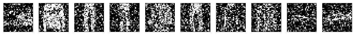

We will use a slightly modified version of the previous convolution autoencoder, the one with larger number of filters in the intermediate layers. This increases the capacity of our model.

input_img = Input(shape=(28, 28, 1))

x = Conv2D(32, (3, 3), activation='relu', padding='same', use_bias=False)(input_img)
x = BatchNormalization(axis=-1)(x)
x = MaxPooling2D((2, 2), padding='same')(x)
x = Conv2D(32, (3, 3), activation='relu', padding='same', use_bias=False)(x)
x = BatchNormalization(axis=-1)(x)
x = MaxPooling2D((2, 2), padding='same')(x)
x = Conv2D(32, (3, 3), activation='relu', padding='same', use_bias=False)(x)
x = BatchNormalization(axis=-1)(x)
encoded = MaxPooling2D((2, 2), padding='same')(x)

x = Conv2D(32, (3, 3), activation='relu', padding='same', use_bias=False)(encoded)
x = BatchNormalization(axis=-1)(x)
x = UpSampling2D((2, 2))(x)
x = Conv2D(32, (3, 3), activation='relu', padding='same', use_bias=False)(x)
x = BatchNormalization(axis=-1)(x)
x = UpSampling2D((2, 2))(x)
x = Conv2D(32, (3, 3), activation='relu', padding='valid', use_bias=False)(x)
x = BatchNormalization(axis=-1)(x)
x = UpSampling2D((2, 2))(x)
decoded = Conv2D(1, (3, 3), activation='sigmoid', padding='same', use_bias=False)(x)

autoencoder = Model(input_img, decoded)
autoencoder.compile(optimizer='rmsprop', loss='binary_crossentropy')

We can now train this for 150 epochs. Notice the change in the training data!

fpath = "weights-dae-{epoch:02d}-{val_loss:.3f}.hdf5"
callbacks = [ModelCheckpoint(fpath, monitor='val_loss', verbose=1, save_best_only=True, mode='min')]
history = autoencoder.fit(x_train_noisy, x_train,
                epochs=150,
                batch_size=256,
                shuffle=True,
                validation_data=(x_test_noisy, x_test),
                callbacks=callbacks)

plot_train_history_loss(history)

The loss has converged to a value of 0.287. Let’s take a look at the results, top row are noisy images and the bottom row are the reconstructed images from the DAE.

autoencoder.load_weights('weights-dae-146-0.287.hdf5')
decoded_imgs = autoencoder.predict(x_test_noisy)
display_reconstructed(x_test_noisy, decoded_imgs, 10)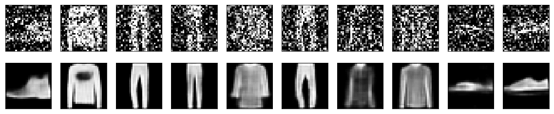

::: callout-pink Sequence-to-Sequence Autoencoders

If your inputs are sequences, rather than 2D images, then you may want to use as encoder and decoder a type of model that can capture temporal structure, such as a LSTM. To build a LSTM-based auto-encoder, first use a LSTM encoder to turn your input sequences into a single vector that contains information about the entire sequence, then repeat this vector $n$ times (where $n$ is the number of time steps in the output sequence), and run a LSTM decoder to turn this constant sequence into the target sequence.

:::

Variational Autoencoders (VAE)Section titled Variational Autoencoders (VAE)

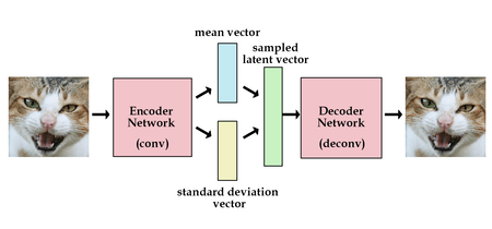
Variational autoencoders (VAE) are stochastic version of the regular autoencoders. It’s a type of autoencoder with added constraints on the encoded representations being learned. More precisely, it is an autoencoder that learns a latent variable model for its input data. So instead of letting your neural network learn an arbitrary function, you are learning the parameters of a probability distribution modeling your data. If you sample points from this distribution, you can generate new input data samples: a VAE is a “generative model”. The cartoon on the side shows a typical architecture of a VAE model. Please refer to the research papers by Kingma et al. and Rezende et al. for a thorough mathematical analysis.

In the probability model framework, a variational autoencoder contains a specific probability model of data $x$ and latent variables $z$ (most commonly assumed as Guassian). We can write the joint probability of the model as $p(x, z) = p(x \vert z)p(z)$ . The generative process can be written as, for each data point $i$ :

Draw latent variables $z_i \sim p(z)$
Draw data point $x_i \sim p(x\vert z)$

In terms of an implementation of VAE, the latent variables are generated by the encoder and the data points are drawn by the decoder. The latent variable hence is a random variable drawn from a posterior distribution, $p(z)$ . To implement the encoder and the decoder as a neural network, you need to backpropogate through random sampling and that is a problem because backpropogation cannot flow through a random node. To overcome this, the reparameterization trick is used. Most commonly, the true posterior distribution for the latent space is assumed to be Guassian. Since our posterior is normally distributed, we can approximate it with another normal distribution, $\mathcal{N}(0, 1)$ .

p(z) \sim \mu + L \mathcal{N}(0, 1)

Here $\mu$ and $L$ are the output of the encoder. Therefore while backpropogation, all we need is partial derivatives w.r.t. $\mu$ , $L$ . In the cartoon above, $\mu$ represents the mean vector latent variable and $L$ represents the standard deviation latent variable.

You can read more about VAE models at Reference 1, Reference 2, Reference 3 and Reference 4.

In more practical terms, VAEs represent latent space (bottleneck layer) as a Guassian random variable (enabled by a constraint on the loss function). Hence, the loss function for the VAEs consist of two terms: a reconstruction loss forcing the decoded samples to match the initial inputs (just like in our previous autoencoders), and the KL divergence between the learned latent distribution and the prior distribution, acting as a regularization term.

\begin{aligned} \min \mathcal{L}(x, x') &= \min E(x, x') \cr &+ KL\big(q(z\vert x)\vert \vert p(z)\big) \end{aligned}

Here, the first term is the reconstruction loss as before (in a typical auto-encoder). The second term is the Kullback-Leibler divergence between the encoder’s distribution, $q(z\vert x)$ and the true posterior $p(z)$ , typically a Guassian.

As typically (especially for images) the binary cross-entropy is used as the reconstruction loss term, the above loss term for the VAEs can be written as,

\begin{aligned} \min{\mathcal{L}(x, x')} &= - \min{\mathbf{E}_{z\sim q(z\vert x)}}\big[ \log p(x' \vert z)\big] \cr &+ KL\big(q(z\vert x) \vert \vert p(z)\big) \end{aligned}

To summarize a typical implementation of a VAE, first, an encoder network turns the input samples $x$ into two parameters in a latent space, z_mean and z_log_sigma. Then, we randomly sample similar points $z$ from the latent normal distribution that is assumed to generate the data, via $z$ = z_mean + exp(z_log_sigma) * $\mathbf{\epsilon}$ , where $\mathbf{\epsilon}$ is a random normal tensor. Finally, a decoder network maps these latent space points back to the original input data.

We can now implement VAE for the fashion MNIST data. To demonstrate its generalization, we will generate two versions: one with MLP and the other with the use of convolution and deconvolution layers.

In the first implementation below, we will be using a simple 2-layer deep encoder and a 2-layer deep decoder. Note the use of the reparameterization trick via the sampling() method and a Lambda layer.

from scipy.stats import norm

from keras.layers import Input, Dense, Lambda, Flatten, Reshape
from keras.layers import Conv2D, Conv2DTranspose
from keras.models import Model
from keras import backend as K
from keras import metrics

batch_size = 128
original_dim = 784
latent_dim = 2
intermediate_dim = 256
epochs = 100
epsilon_std = 1.0


x = Input(shape=(original_dim,))
h = Dense(intermediate_dim, activation='relu')(x)
z_mean = Dense(latent_dim)(h)
z_log_var = Dense(latent_dim)(h)


def sampling(args):
    z_mean, z_log_var = args
    epsilon = K.random_normal(shape=(K.shape(z_mean)[0], latent_dim), mean=0.,
                              stddev=epsilon_std)
    return z_mean + K.exp(z_log_var / 2) * epsilon

# note that "output_shape" isn't necessary with the TensorFlow backend
z = Lambda(sampling, output_shape=(latent_dim,))([z_mean, z_log_var])

# to reuse these later
decoder_h = Dense(intermediate_dim, activation='relu')
decoder_mean = Dense(original_dim, activation='sigmoid')
h_decoded = decoder_h(z)
x_decoded_mean = decoder_mean(h_decoded)

# instantiate VAE model
vae = Model(x, x_decoded_mean)

As described above, we need to include two loss terms, binary cross entropy as before and the KL divergence between the encoder latent variable distribution (calculated using the reparameterization trick) and the true posterior distribution, a normal distribution!

# Compute VAE loss
xent_loss = original_dim * metrics.binary_crossentropy(x, x_decoded_mean)
kl_loss = - 0.5 * K.sum(1 + z_log_var - K.square(z_mean) - K.exp(z_log_var), axis=-1)
vae_loss = K.mean(xent_loss + kl_loss)

vae.add_loss(vae_loss)
vae.compile(optimizer='rmsprop')

we can now load the fashion MNIST dataset, normalize it and reshape it to correct dimensions so that it can be used with our VAE model.

# train the VAE on fashion MNIST images
(x_train, y_train), (x_test, y_test) = fashion_mnist.load_data()

x_train = x_train.astype('float32') / 255.
x_test = x_test.astype('float32') / 255.
x_train = x_train.reshape((len(x_train), np.prod(x_train.shape[1:])))
x_test = x_test.reshape((len(x_test), np.prod(x_test.shape[1:])))

We will now train our model for 100 epochs.

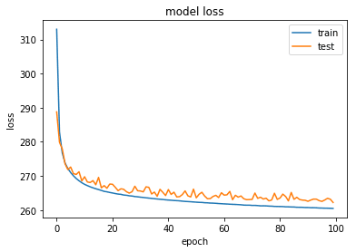
history = vae.fit(x_train,
        shuffle=True,
        epochs=epochs,
        batch_size=batch_size,
        validation_data=(x_test, None))

plot_train_history_loss(history)

Below is the loss for the training and the validation datasets during training epochs. We find that loss has converged in 100 epochs without any sign of over fitting.

Because our latent space is two-dimensional, there are a few cool visualizations that can be done at this point. One is to look at the neighborhoods of different classes on the latent 2D plane:

# build a model to project inputs on the latent space
encoder = Model(x, z_mean)

# display a 2D plot of the digit classes in the latent space
def plot_latentSpace(encoder, x_test, y_test, batch_size):
    x_test_encoded = encoder.predict(x_test, batch_size=batch_size)
    plt.figure(figsize=(6, 6))
    plt.scatter(x_test_encoded[:, 0], x_test_encoded[:, 1], c=y_test, cmap='tab10')
    plt.colorbar()
    plt.show()

plot_latentSpace(encoder, x_test, y_test, batch_size)

Each of these colored clusters is a type of the fashion item. Close clusters are items that are structurally similar (i.e. items that share information in the latent space). We cal also look at this plot from a different perspective: the better our VAE model, the separation between very dissimilar fashion items would be larger among their clusters!

Because the VAE is a generative model (as described above), we can also use it to generate new images! Here, we will scan the latent plane, sampling latent points at regular intervals, and generating the corresponding image for each of these points. This gives us a visualization of the latent manifold that “generates” the fashion MNIST images.

# generator that can sample from the learned distribution
decoder_input = Input(shape=(latent_dim,))
_h_decoded = decoder_h(decoder_input)
_x_decoded_mean = decoder_mean(_h_decoded)
generator = Model(decoder_input, _x_decoded_mean)

def plot_generatedImages(generator):
    # D manifold of the fashion images
    n = 15  # figure with 15x15 images
    image_size = 28
    figure = np.zeros((image_size * n, image_size * n))
    # linearly spaced coordinates on the unit square were transformed through the # inverse CDF (ppf) of the Gaussian
    # to produce values of the latent variables z, since the prior of the latent
    # space is Gaussian
    grid_x = norm.ppf(np.linspace(0.005, 0.995, n))
    grid_y = norm.ppf(np.linspace(0.005, 0.995, n))

    for i, yi in enumerate(grid_x):
        for j, xi in enumerate(grid_y):
            z_sample = np.array([[xi, yi]])
            x_decoded = generator.predict(z_sample)
            digit = x_decoded[0].reshape(image_size, image_size)
            figure[i * image_size: (i + 1) * image_size,
                   j * image_size: (j + 1) * image_size] = digit

    plt.figure(figsize=(10, 10))
    plt.imshow(figure, cmap='Greys_r')
    plt.show()

plot_generatedImages(generator)

We find our model has done only a so-so job in generating new images. Still, given the simplicity and very small amount of simple code we had to write, this is still quite incredible.

We can next build a more realistic VAE using conv and deconv layers. Below is the full code to build and train the model.

# input image dimensions
img_rows, img_cols, img_chns = 28, 28, 1
# number of convolutional filters to use
filters = 64
# convolution kernel size
num_conv = 3

batch_size = 128
if K.image_data_format() == 'channels_first':
    original_img_size = (img_chns, img_rows, img_cols)
else:
    original_img_size = (img_rows, img_cols, img_chns)
latent_dim = 2
intermediate_dim = 128
epsilon_std = 1.0
epochs = 150

x = Input(shape=original_img_size)
conv_1 = Conv2D(img_chns,
                kernel_size=(2, 2),
                padding='same', activation='relu')(x)
conv_2 = Conv2D(filters,
                kernel_size=(2, 2),
                padding='same', activation='relu',
                strides=(2, 2))(conv_1)
conv_3 = Conv2D(filters,
                kernel_size=num_conv,
                padding='same', activation='relu',
                strides=1)(conv_2)
conv_4 = Conv2D(filters,
                kernel_size=num_conv,
                padding='same', activation='relu',
                strides=1)(conv_3)
flat = Flatten()(conv_4)
hidden = Dense(intermediate_dim, activation='relu')(flat)

z_mean = Dense(latent_dim)(hidden)
z_log_var = Dense(latent_dim)(hidden)


def sampling(args):
    z_mean, z_log_var = args
    epsilon = K.random_normal(shape=(K.shape(z_mean)[0], latent_dim),
                              mean=0., stddev=epsilon_std)
    return z_mean + K.exp(z_log_var) * epsilon

# note that "output_shape" isn't necessary with the TensorFlow backend
# so you could write `Lambda(sampling)([z_mean, z_log_var])`
z = Lambda(sampling, output_shape=(latent_dim,))([z_mean, z_log_var])

# we instantiate these layers separately so as to reuse them later
decoder_hid = Dense(intermediate_dim, activation='relu')
decoder_upsample = Dense(filters * 14 * 14, activation='relu')

if K.image_data_format() == 'channels_first':
    output_shape = (batch_size, filters, 14, 14)
else:
    output_shape = (batch_size, 14, 14, filters)

decoder_reshape = Reshape(output_shape[1:])
decoder_deconv_1 = Conv2DTranspose(filters,
                                   kernel_size=num_conv,
                                   padding='same',
                                   strides=1,
                                   activation='relu')
decoder_deconv_2 = Conv2DTranspose(filters,
                                   kernel_size=num_conv,
                                   padding='same',
                                   strides=1,
                                   activation='relu')
if K.image_data_format() == 'channels_first':
    output_shape = (batch_size, filters, 29, 29)
else:
    output_shape = (batch_size, 29, 29, filters)
decoder_deconv_3_upsamp = Conv2DTranspose(filters,
                                          kernel_size=(3, 3),
                                          strides=(2, 2),
                                          padding='valid',
                                          activation='relu')
decoder_mean_squash = Conv2D(img_chns,
                             kernel_size=2,
                             padding='valid',
                             activation='sigmoid')

hid_decoded = decoder_hid(z)
up_decoded = decoder_upsample(hid_decoded)
reshape_decoded = decoder_reshape(up_decoded)
deconv_1_decoded = decoder_deconv_1(reshape_decoded)
deconv_2_decoded = decoder_deconv_2(deconv_1_decoded)
x_decoded_relu = decoder_deconv_3_upsamp(deconv_2_decoded)
x_decoded_mean_squash = decoder_mean_squash(x_decoded_relu)

# instantiate VAE model
vae = Model(x, x_decoded_mean_squash)

# define the loss function
xent_loss = img_rows * img_cols * metrics.binary_crossentropy(
    K.flatten(x),
    K.flatten(x_decoded_mean_squash))
kl_loss = - 0.5 * K.sum(1 + z_log_var - K.square(z_mean) - K.exp(z_log_var), axis=-1)
vae_loss = K.mean(xent_loss + kl_loss)
vae.add_loss(vae_loss)

vae.compile(optimizer='rmsprop')

# load the data
(x_train, _), (x_test, y_test) = fashion_mnist.load_data()

x_train = x_train.astype('float32') / 255.
x_train = x_train.reshape((x_train.shape[0],) + original_img_size)
x_test = x_test.astype('float32') / 255.
x_test = x_test.reshape((x_test.shape[0],) + original_img_size)

# train the VAE model
history = vae.fit(x_train,
        shuffle=True,
        epochs=epochs,
        batch_size=batch_size,
        validation_data=(x_test, None))

plot_train_history_loss(history)

Similar to the case of simple VAE model, we can look at the neighborhoods of different classes on the latent 2D plane:

# project inputs on the latent space
encoder = Model(x, z_mean)
plot_latentSpace(encoder, x_test, y_test, batch_size)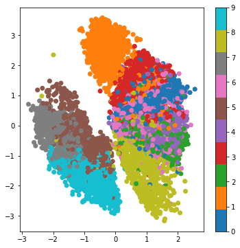

We can now see that the separation between different class of images are larger than the simple MLP based VAE model.

Finally, we can now generate new images from our, hopefully, better VAE model.

# generator that can sample from the learned distribution
decoder_input = Input(shape=(latent_dim,))
_hid_decoded = decoder_hid(decoder_input)
_up_decoded = decoder_upsample(_hid_decoded)
_reshape_decoded = decoder_reshape(_up_decoded)
_deconv_1_decoded = decoder_deconv_1(_reshape_decoded)
_deconv_2_decoded = decoder_deconv_2(_deconv_1_decoded)
_x_decoded_relu = decoder_deconv_3_upsamp(_deconv_2_decoded)
_x_decoded_mean_squash = decoder_mean_squash(_x_decoded_relu)
generator = Model(decoder_input, _x_decoded_mean_squash)

plot_generatedImages(generator)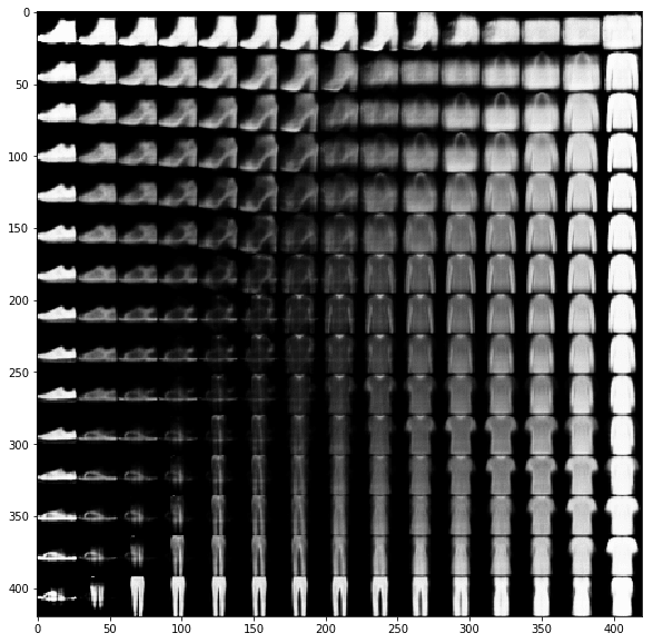

Usage of AutoencodersSection titled Usage of Autoencoders

Most common uses of Autoenoders are:

Dimensionality Reduction: Dimensionality reduction was one of the first applications of representation learning and deep learning. Lower-dimensional representations can improve performance on many tasks, such as classification. Models of smaller spaces consume less memory and runtime. The hints provided by the mapping to the lower-dimensional space aid generalization. Due to non-linear nature, autoencoders tend to perform better than traditional techniques like PCA, kernel PCA etc.
Denoising and Transformation: You can distort the data and add some noise in it before feeding it to DAEs. This can help in generalizing over the test set. AEs are also useful in image transformation tasks, eg. document cleaning, applying color to images, medical image segmentation using U-net, a variant of autoencoders etc.

Information Retrieval: the task of finding entries in a database that resemble a query entry. This task derives the usual benefits from dimensionality reduction that other tasks do, but also derives the additional benefit that search can become extremely efficient in certain kinds of low-dimensional spaces.
In Natural Language Processing
- Word Embeddings
- Machine Translation
- Document Clustering
- Sentiment Analysis
- Paraphrase Detection
Image/data Generation: We saw theoretical details of generative nature of VAEs above. See this blog post by openAI for a detailed review of image generation.
Anamoly detection: For highly imbalanced data (like credit card fraud detection, defects in manufacturing etc.) you may have sufficient data for the positive class and very few or no data for the negative class. In such situations, you can train an AE on your positive data and learn features and then compute reconstruction error on the training set to find a threshold. During testing, you can use this threshold to reject those test instances whose values are greater than this threshold. However, optimizing the threshold that can generalize well on the unseen test cases is challenging. VAEs have been used as alternative for this task, where reconstruction error is probabilistic and hence easier to generalize. See this article by FICO where they use autoencoders for detecting anomalies in credit scores.

This is it! its been quite a long article. Hope this is helpful to some of you. Please let me know via comments below if any particular issues/concepts you would like me to go over in more details. I would also love to know if any particular topic in machine/deep learning you would like me to cover in future posts.

Deep Learning, Algorithms