Understanding Boosted Trees Models

In the previous post, we learned about tree based learning methods - basics of tree based models and the use of bagging to reduce variance. We also looked at one of the most famous learning algorithms based on the idea of bagging- random forests.

In this post, we will look into the details of yet another type of tree-based learning algorithms: boosted trees.

BoostingSection titled Boosting

Boosting, similar to Bagging, is a general class of learning algorithm where a set of weak learners are combined to get strong learners.

For classification problems, a weak learner is defined to be a classifier which is only slightly correlated with the true classification (it can label examples better than random guessing). In contrast, a strong learner is a classifier that is arbitrarily well-correlated with the true classification.

Recall that bagging involves creating multiple copies of the original training data set via bootstrapping, fitting a separate decision tree to each copy, and then combining all of the trees in order to create a single predictive model. Notably, each tree is built on a bootstrap data set, independent of the other trees.

In contrast, in Boosting, the trees are grown sequentially: each tree is grown using information from previously grown trees. Boosting does not involve bootstrap sampling; instead each tree is fit on a modified version of the original data set.

Unlike fitting a single large decision tree to the data, which amounts to fitting the data hard and potentially overfitting, the boosting approach instead learns slowly. Given the current model, a decision tree is fit to the residuals from the model. That is, a tree is fit using the current residuals, rather than the outcome as the response.

The above concept of additively fitting weak learners to get a strong learner is not limited to tree based methods. In fact, we can choose these weak learners to be any model of our choice. In practice, however, decision trees or sometimes linear models are the most common choices. In this post, we will be focusing mainly on boosted trees - i.e. our choice of weak learners would be decision trees. Boosted trees are one of the most used models in on-line machine learning competitions like Kaggle.

Let us consider the case of boosted trees more rigorously. In particular, we will look at the case of boosted decision trees for regression problems. To begin, set the resultant model $\hat{F}(x) = 0$ and residual of the training response as the training target $y$ . Now Sequentially, for steps $b=1,2\ldots,B$ update $\hat{F}(x)$ as follows: $\hat{F}(x)\leftarrow \hat{F}(x) + \lambda_b \hat{f}^{b}(x)$ , where $\hat{f}^{b}(x)$ is a decision tree learner fit on $(X, r)$ with $d$ splits (or $d+1$ terminal nodes) and $\lambda_b$ is a weighting parameter. Also update residuals, $r$ as, $r \leftarrow r - \lambda_b \hat{f}^{b}(x)$ . At the end of $B$ steps, we will get the final model as $\hat{F}(x) = \sum_{b=1}^{B}\lambda_b\hat{f}^{b}(x)$ .

The above algorithm of boosted is quite generic. One can come with several strategies for how the decision trees are grown and fit on residuals, and for the choice of the weighting parameter $\lambda$ . Therefore, there are various boosting methods. Some common examples are:

In this post, we will focus specifically on two of the most common boosting algorithms, AdaBoost and Gradient Boosting.

Adaptive Boosting (AdaBoost)Section titled Adaptive Boosting (AdaBoost)

Adaptive Boosting or AdaBoost refers to a particular formulation of boosting where the idea of residual learning is implemented through the concept of sample weights. In particular, at any iteration, $b$ , all training samples have a weight $w_i^b$ $\forall i = 1, \ldots N$ , which is equal to the current error $E(\hat{f}(x_i))$ . The decision tree $\hat{f}^{b}(x)$ is fit to minimize the error $E_b = \sum_{i=1}^{N}{E\big(\hat{F}(x) + \lambda_b \hat{f}^{b}(x)\big)}$ . AdaBoost uses an exponential error/loss function: $E(\hat{F}(x_i)) = e^{-y_i \hat{F}(x_i)}$ . The choice of the error function, $E()$ , also determines the way weights $w_i^b$ and the weighting parameter $\lambda_b$ are updated at different steps. A neat mathematical derivation of these quantities for the case of binary classification can be found at the Wiki article.

In particular case of the classification problems, we can also think of AdaBoost to be an algorithm where at any step, the misclassified samples get a higher weight than the correctly classified samples. The weights attached to samples are used to inform the training of the weak learner, in this case, decision trees to be grown in a way that favor splitting the sets of samples with high weights.

In practice, the above definition of the AdaBoost model is modified to include a learning rate term, $\gamma$ , as a regularization term that shrinks the contribution of all of the models. In particular, the model is updated as, $\hat{F}(x) \leftarrow \hat{F}(x) + \gamma \lambda_b \hat{f}^{b}(x)$ . The main tuning parameters of AdaBoost are, the learning rate $\gamma$ , number of estimators $B$ , and decision tree related parameters like depth of trees $d$ , and number of samples per split etc.

AdaBoost in Python

The python scikit-learn library implementations of AdaBoost (AdaBoostClassifier and AdaBoostRegressor) are based on a modified version of the AdaBoost algorithms, AdaBoost SAMME and SAMME.R. Stage-wise Additive Modeling using a Multi-class Exponential loss function (SAMME) algorithm provides an extension of AdaBoost for the case of multi-class classification. The SAMME.R (R for real) variation of the algorithm is for prediction of weighted probabilities rather than the class itself.

AdaBoost Classifier in PythonSection titled AdaBoost Classifier in Python

Recall the US income data that we used in the previous based post on tree based methods. In summary, in this dataset, we are required to predict the income range of adults ( $<=50K$ or $>50K$ ) based on following features: Race, Sex, Education, Work Class, Capital Loss, Capital Gain, Relationship, Marital Status, Age Group, Occupation and Hours of Work per Week. We have already seen that, with the best decision tree model, we were able to achieve a prediction accuracy of 85.9%. With the use of random forest models, we were able to increase the accuracy to 86.6%.

Let us try to solve the same problem using AdaBoost classifier from scikit-learn module. Please have a look at the previous post on tree-based methods to understand the EDA and preparation of the data.

from sklearn.ensemble import AdaBoostClassifier
aclf = AdaBoostClassifier(DecisionTreeClassifier(max_depth=5), n_estimators=100)
aclf.fit(x_train, y_train)
aclf.score(x_test, y_test)

Without any parameter tuning, we see an accuracy of 85.54%!

Genetic Algorithms for Parameter Search

Once the number of hyper-parameters and the range of those parameter in models becomes large, the time required to find the best parameters becomes exponentially large using simple grid search. Instead of trying out every possible combination of parameters, we can evolve only the combinations that give the best results using Genetic Algorithms. A scikit-learn friendly implementation of this can be found in the sklearn-deap library. In many of the examples below we will be using this library to search for best model parameters.

The genetic algorithm itself has three main parameters: population size, tournament size and no. of generations. Typically, for the problem of parameter search, we can use a population of 10-15 per hyper-parameter. The tournament size parameter affects the diversity of population being considered in future generation. This roughly translates into global vs local optimization for parameter search. In other words, if the tournament size is too large, we will have higher chance of getting a solution that is from local minima. A typical value of 0.1 times the population works well for the exercise of finding optimal model parameters. The number of generation decides the convergence of genetic algorithms. A larger value leads to better convergence but requires larger computation time.

Let us try using genetic algorithm to find optimal model parameters for AdaBoost classifier.

from evolutionary_search import EvolutionaryAlgorithmSearchCV

parameters = {
     'base_estimator__max_features':(11, 9, 6),
     'base_estimator__max_depth':(1, 2, 4, 8),
     'base_estimator__min_samples_split': (2, 4, 8),
     'base_estimator__min_samples_leaf': (16, 12, 8, 4),
     'n_estimators': (50, 100, 200, 500),
     'learning_rate': (1, 0.1, 0.01, 10)
}

clf2 = EvolutionaryAlgorithmSearchCV(estimator=aclf,
        params=parameters,
        scoring="accuracy",
        cv=5,
        verbose=1,
        population_size=200,
        gene_mutation_prob=0.10,
        gene_crossover_prob=0.5,
        tournament_size=10,
        generations_number=100,
        n_jobs=8)
clf2.fit(x_train, y_train)

This should take about 50 minutes on a reasonable desktop machine! We can now use the best parameters from this and create a new AdaBoost classifier.

aclf = AdaBoostClassifier(
    ecisionTreeClassifier(max_depth=4,
        max_features=11,
        min_samples_leaf=4,
        min_samples_split=2),
    n_estimators=100,
    learning_rate=0.1)
aclf.fit(x_train, y_train)
aclf.score(x_test, y_test)

We see a significant improvement in our results with an accuracy of 87.06% on the testing data!

Given our data is highly imbalanced, let us look at the confusion matrix of our model on the test data. Note that we are using the confusion_matrix() method from the previous post on tree based methods.

y_pred = aclf.predict(x_test)
cfm = confusion_matrix(y_test, y_pred, labels=[0, 1])
plt.figure(figsize=(10,6))
plot_confusion_matrix(cfm, classes=["<=50K", ">50K"], normalize=True)

We find that our model has a much better predictive power (94.1%) for the dominant class ( $<=50K$ ), while it has prediction rate of only 64.2% for the other class.

Gradient BoostingSection titled Gradient Boosting

The approach used in the case of AdaBoost can be also viewed as an exponential loss minimization approach. Let us look at this mathematically for the case of a generic loss function, $L\big(y,\hat{F}(x)\big)$ . The goal of the method is to find an $\hat{F}(x)$ that minimizes the average value of the loss function $L\big(y,\hat{F}(x)\big)$ on the training set. This can be achieved by starting with a constant function $\hat{F_0}(x)$ , and incrementally expanding it in a greedy fashion as follows:

\begin{gathered} \hat{F_0}(x) = \mathop{\arg\min}\limits_{\gamma} \sum_{i=1}^{N} L\big(y,\gamma \big) \cr \hat{F_b}(x) = \hat{F}_{b-1}(x) + \cr \mathop{\arg\min}\limits_{f \in \mathcal{H}} \sum_{i=1}^{N} L\big(y,\hat{F}_{b-1}(x) + f(x) \big) \cr \text{, for } b=1,2,\ldots, B \end{gathered}

where $f(x) \in \mathcal{H}$ refers to base learners, in this case tree models. The problem with this set up is that, it is computationally infeasible to choose optimal $f(x)$ at every step for an arbitrary loss function $L\big(y,\hat{F}(x)\big)$ .

However, this can be simplified using a steepest descent approach. In this approach, at any step the decision tree model is trained on the pseudo-residuals, rather than residuals. The approach can be described in the following algorithm:

Initialize model as, $\hat{F_0}(x) = \mathop{\arg\min}\limits_{\gamma} \sum_{i=1}^{N} L\big(y,\gamma \big)$
for steps $b=1,2,\ldots, B$ :
- compute pseudo-residuals as: $r_{ib} = -\Bigg[ \frac{\partial{L\big(y_i, \hat{F}_{b-1}(x_i)\big)}}{\partial{\hat{F}_{b-1}(x_i)}} \Bigg]$
- Fit a decision tree $\hat{f^b}(x)$ to pseudo-residuals, i.e. train it using the training set $(x_i, r_{ib})_{i=1}^N$
- Compute multiplier $\gamma_b$ using line search, where $0<\nu<1$ is the learning rate parameter $\gamma_b = \mathop{\arg\min}\limits_{\gamma} \sum_{i=1}^N L\big(y_i, \hat{F}_{b-1}(x) + \nu \gamma \hat{f^b}(x)\big)$
- update the model $\hat{F_b}(x) = \hat{F}_{b-1}(x) + \nu \gamma_b \hat{f^b}(x)$

In most real implementations of gradient boosted trees, rather than an individual tree weighing parameter $\gamma_b$ , different parameters are used at different splits, $\gamma_{jb}$ . If you recall from the last post, a decision tree model corresponds to diving the feature space in multiple rectangular regions and hence it can be represented as,

\hat{f^b}(x) = \sum_{j=1}^{J} k_{jb} I\big(x\in R_{jb}\big)

where, $J$ is the number of terminal nodes (leaves), $I\big(x\in R_{jb}\big)$ is an indicator function which is 1 if $x\in R_{jb}$ and $k_{jb}$ is the prediction in $j^{th}$ leaf. Now, we can replace $\hat{f^b}(x)$ in above algorithm and replace $\gamma_b$ for the whole tree by $\gamma_{jb}$ per terminal node (leaf).

\hat{F_b}(x) = \hat{F}_{b-1}(x) + \nu \sum_{j=1}^{J_b} \gamma_{jb} I\big(x\in R_{jb}\big)

where $\gamma_{jb}$ is given by the following line search,

\gamma_{jb} = \mathop{\arg\min}\limits_{\gamma} \sum_{x_i \in R_{jb}} L\big(y_i, \hat{F}_{b-1}(x) + \gamma \big)

Here $J$ refers to the number of terminal nodes (leaves) in any of constituent decision trees. A value of $J_b =2$ , i.e. decision stumps means no interactions among feature variables are considered. With a value of $J_b=3$ the model may include effects of the interaction between up to two variables, and so on. Typically a value of $4 \le J_b \le 8$ work well for boosting.

Regularization of Gradient Boosted TreesSection titled Regularization of Gradient Boosted Trees

Gradient Boosted Trees can be regularized by multiple approaches. Some common approaches are:

Shrinkage / Learning Rate: For each gradient step, the step magnitude is multiplied by a factor between 0 and 1 called a learning rate ( $0 <\nu < 1$ ). In other words, each gradient step is shrunken by some factor $\nu$ . The rational for this to work as a regularization parameter has never been clear to me. My personal take is the shrinkage enables us to use a different prior. Telgarsky et al. provide a mathematical proof that shrinkage makes gradient boosting to produce an approximate maximum margin classifier, i.e. a classifier which is able to maximize the associated distance from the decision boundary for each example.
Sub-Sampling: Motivated by the bagging method, at each iteration of the algorithm, a decision tree is fit on a subsample of the training set drawn at random without replacement. Also, like in bagging, sub-sampling allows one to define an out-of-bag error of the prediction performance improvement by evaluating predictions on those observations which were not used in the building of the next base learner. Out-of-bag estimates help avoid the need for an independent validation dataset, but often underestimate actual performance improvement and the optimal number of iterations.
Minimum sample size for splitting trees, and Minimum sample size for tree leaves: It is used in the tree building process by ignoring any splits that lead to nodes containing fewer than this number of training set instances. Imposing this limit helps to reduce variance in predictions at leaves.
The number of trees or Boosting Iterations, $B$ Increasing $B$ reduces the error on training set, but setting it too high may lead to over-fitting. An optimal value of $B$ is often selected by monitoring prediction error on a separate validation data set.
Sampling Features: We can apply the idea of randomly choosing small subsets of features for different trees, as in the case of Random Forest models.

scikit-learn ImplementationSection titled scikit-learn Implementation

scikit-learn provides a simple and generic implementation of the above described algorithm that is valid of different types of loss functions. Below is a simple implementation for the case of income data.

from sklearn.ensemble import GradientBoostingClassifier

params = {'n_estimators': 200, 'max_depth': 4, 'subsample': 0.75,
          'learning_rate': 0.1, 'min_samples_leaf': 4, 'random_state': 3}
gclf = GradientBoostingClassifier(**params)

gclf.fit(x_train, y_train)
gclf.score(x_test, y_test)

Turns out we have got a quite good model just by chance! This has an accuracy of 87.11% on our test data!

We could try finding optimal parameters for this as before. However, in my experience this is a very academic implementation of boosted trees. Other implementation like XGBoost, LightGBM and CatBoost are more optimized implementations and hence we will focus our tuning for some of these libraries only.

XGBoostSection titled XGBoost

The biggest drawback of the gradient boosting trees is that the algorithm is quite sequential in nature and hence are very slow and they can not take advantage of advanced computing features for parallelization like multiple threads and cores, GPU etc.

XGBoost is a python (C++ and R as well) library that provides an optimized implementation of gradient boosted trees. It uses various tricks like regularization of number of leaves and leaf weights, sparsity aware split finding, column block for parallel learning and cache-aware access. Using these tricks the implementation provides a parallelized efficient version of the algorithm. The details of these can be found here. XGBoost is one of the most famous machine learning libraries used in on-line machine learning competitions like Kaggle.

Regularization

Apart from regular gradient boosted trees, XGBoost provides two additional types of regularization, by adding $L_1$ constraints on number of leaves ( $J_b$ ) and $L_2$ constraints on the leaf weights ( $\gamma_{jb}$ ) to the loss function. Mathematically, The loss function is modified as follows (Loss Term at step b):

\sum_{i=1}^{N} L\big( y_i, \hat{F_b}(x_i) \big) + \sum_{k=1}^b \Big (\eta J_k + \frac{1}{2} \lambda \left\lVert \gamma_{jk} \right\rVert^2 \Big )

Here, the second term in the loss function, penalizes the complexity of the model, i.e. decision tree functions.

Additional Weak Learners: Apart from decision trees, XGBoost also supports linear models and DART (decision trees with dropout) as weak learners. In the DART algorithm, only a subset of available trees are considered in calculating the pseudo-residuals on which the new trees are fit.

XGBoost has many parameters that control the fitting of the model. Below are some of the relevant parameters and tuning them would be helpful in the most common cases. Please note that original XGBoost library parameters might have a different name than before, since I am using the scikit-learn API parameter names below.

max_depth (default=3) : Maximum depth of a tree, increase this value will make the model more complex / likely to be over-fitting. A value of 0 indicates no limit. A Typical Value in the range of 2-10 can be used for model optimization.
n_estimators (default=100) : The number of boosting steps to perform. This can also be seen as number of trees to be used in the boosted model. This number is inversely proportional to the learning*rate (eta) parameter, i.e. if we use a smaller value of learning_rate, n_estimators has to be made larger. A Typical Value in the range of $\ge 100$ can be used for model optimization. However, it is best to used XGBoost built-in cv() method to find this parameter (See the example ahead).
min_child_weight (default=1) : The minimum sum of instance weight needed in a child node. If the tree partition step results in a leaf node with the sum of instance weight less than the min_child_weight, then any further partitioning will be stopped. The larger the value of this parameter, the more conservative the algorithm will be. A Typical Value in the range of 1-10 can be used for model optimization*.
learning_rate (default=0.1) : The step size shrinkage used to prevent over-fitting. After each boosting step, we can directly get the weights of new features. and the learning_rate parameter (also referred as eta in regular XGBoost API) shrinks the feature weights to make the boosting process more conservative (See above formulation of Gradient Boosted Trees for mathematical details). A Typical Value in the range of 0.001-0.3 can be used for model optimization.
gamma (default=0) : (Also referred as min_split_loss in regular XGBoost API) The minimum loss reduction required to make a further partition on a leaf node of the tree. The larger, the more conservative the algorithm will be. The value of this parameter depends on the type of loss function being used. A Typical Value in the range of 0.0-0.7 can be used for model optimization.
reg_alpha (default=0) : (Also referred as alpha in regular XGBoost API) L1 regularization term on weights, increasing this value will make model more conservative (see XGBoost paper for mathematical details). A Typical Value in the range of 0-1 can be used for model optimization.
reg_lambda (default=1) : (Also referred as lambda in regular XGBoost API) L2 regularization term on weights, increasing this value will make model more conservative (see XGBoost paper for mathematical details). A Typical Value in the range of 0-1 can be used for model optimization.
subsample (default=1) : Subsample ratio of the training instance. Setting it to 0.5 means that XGBoost randomly collected half of the data instances to grow trees. This parameter is used to prevent over-fitting. A Typical Value in the range of 0.5-1.0 can be used for model optimization.
colsample_bytree (default=1) : Subsample ratio of columns when constructing each tree. Similar to Random Forest models, models tend to be more generalizable, if a number between 0 and 1 is used. A Typical Value in the range of 0.5-1.0 can be used for model optimization.
scale_pos_weight (default=1) : Controls the balance of positive and negative class weights, useful for unbalanced class problems. A typical value to consider: sum(negative cases) / sum(positive cases).

Apart from above set of parameters, there are several parameters that should also be considered while tuning. Some examples of such parameters are: objective (objective function/ loss function to use, depends on problem, for eg. binary vs. multi-class classification), tree_method (The tree construction algorithm used in XGBoost(see description in the paper), random_state (seed for random number generator), n_jobs (number of threads to use to train the model) and many other parameters related to different types of tree methods used. This article can be used as a good general reference for tuning XGBoost models.

Let us tune XGBoost model for our problem of income prediction. A simple sklearn API implementation can be used as below.

import xgboost as xgb

params = {
    'n_estimators': 100,
    'max_depth': 6,
    'subsample': 0.75,
    'learning_rate': 0.1,
    'min_samples_split': 2,
    'min_samples_leaf': 8,
    'random_state': 32,
    'objective': 'binary:logistic',
    'n_jobs': 8
    }
xclf = xgb.XGBClassifier(**params)

xclf.fit(x_train, y_train)
xclf.score(x_test, y_test)

With this reasonable guess of parameters based on previous models, we already see an accuracy of 86.75%.

Let us try to find the optimal parameters for the XGBoost model. If we simply try to do a brute force grid search, it can be computationally very expensive and unreasonable on a desktop. Here is a sample parameters list that can give us an idea of what such a grid search could look like.

independent_params = {
    'random_state': 32,
    'objective': 'binary:logistic',
    'n_jobs': 8,
}
params = {
    'n_estimators': (100, 200, 400, 800, 1000),
    'max_depth': (4, 6, 8),
    'subsample': (0.75, 0.8, 0.9, 1.0),
    'learning_rate': (0.1, 0.01, 0.05),
    'colsample_bytree': (0.75, 0.8, 0.9, 1.0),
    'min_child_weight': range(1,6,2),
    'reg_alpha': [i/10.0 for i in range(0,5)],
    'gamma':[i/10.0 for i in range(0,5)],
    'reg_lambda': (1, 0.1, 10)
    }

If we try to do a grid search of this with 5-fold cross validation, it will involve a whopping 0.81 million model training calls! And, even this will not be enough, as we will need additional model training steps to fine-tune our parameter search for finer and/or different range of parameters. Clearly, we need a different approach to solve this.

I will take an approach of optimizing different set of parameters in batches. To begin, we will choose a fixed learning rate of 0.1, and n_estimators=200. We will try to find only tree related parameters (i.e. max_depth, gamma, subsample and colsample_bytree) using grid search or genetic algorithm.

ind_params = {
    'random_state': 32,
    'objective': 'binary:logistic',
    'n_estimators': 200,
    'learning_rate': 0.1,
}
params = {
    'max_depth': (4, 6, 8),
    'subsample': (0.75, 0.8, 0.9, 1.0),
    'colsample_bytree': (0.75, 0.8, 0.9, 1.0),
    'gamma': [i/10 for i in range(0,5)]
}

clf2 = EvolutionaryAlgorithmSearchCV(
        estimator=xgb.XGBClassifier(**ind_params),
        params=params,
        scoring="accuracy",
        cv=5,
        verbose=1,
        population_size=60,
        gene_mutation_prob=0.10,
        gene_crossover_prob=0.5,
        tournament_size=5,
        generations_number=100,
        n_jobs=8)
clf2.fit(x_train, y_train)

This gives us the following optimal values for different parameters:

Best individual is: {'max_depth': 6, 'subsample': 1.0, 'colsample_bytree': 0.8, 'gamma': 0.2}
with fitness: 0.8710727557507447

We can do a finer grid search to get more precise values. For this exercise, let us move on to the next stage of parameter tuning of XGBoost.

XGBoost provides an optimized version of cross validation using cv() method which supports early stopping to give us optimal value of n_estimators.

xgb1 = xgb.XGBClassifier(
 learning_rate =0.1,
 n_estimators=10000,
 max_depth=6,
 min_child_weight=1,
 gamma=0.2,
 subsample=1.0,
 colsample_bytree=0.8,
 objective= 'binary:logistic',
 n_jobs=8,
 scale_pos_weight=1,
 random_state=32)
xgb_param = xgb1.get_xgb_params()
xgtrain = xgb.DMatrix(x_train, label=y_train)
cvresult = xgb.cv(xgb_param, xgtrain, num_boost_round=xgb1.get_params()['n_estimators'], nfold=5, metrics='auc', early_stopping_rounds=50)

print("Number of Predicted n_estimators = ", cvresult.shape[0])

This gives us a value of n_estimators = 206. We will now use these parameters to search for the next set of tree building parameters: max_depth and min_child_weight.

params = {
 'max_depth':range(3,10,2),
 'min_child_weight':range(1,6,2)
}

ind_params = {'learning_rate': 0.1,
 'n_estimators': 206,
 'gamma': 0.2,
 'subsample': 1.0,
 'colsample_bytree': 0.8,
 'objective': 'binary:logistic',
 'random_state': 32}

clf2 = EvolutionaryAlgorithmSearchCV(
        estimator=xgb.XGBClassifier(**ind_params),
        params=params,
        scoring="accuracy",
        cv=5,
        verbose=1,
        population_size=30,
        gene_mutation_prob=0.10,
        gene_crossover_prob=0.5,
        tournament_size=5,
        generations_number=100,
        n_jobs=8
    )
clf2.fit(x_train, y_train)

The optimal set of parameters found by this are:

Best individual is: {'max_depth': 7, 'min_child_weight': 1}
with fitness: 0.8712877368631184

We can now use these parameters as fixed values and optimize regularization parameters: reg_alpha and reg_lambda.

ind_params = {'learning_rate': 0.1,
 'n_estimators': 206,
 'gamma': 0.2,
 'subsample': 1.0,
 'colsample_bytree': 0.8,
 'objective': 'binary:logistic',
 'random_state': 32,
 'max_depth': 7,
 'min_child_weight': 1}

params = {'reg_alpha':[0, 0.001, 0.005, 0.01, 0.05], 'reg_lambda':[0.01, 0.1, 1, 10, 100]}

clf2 = EvolutionaryAlgorithmSearchCV(
        estimator=xgb.XGBClassifier(**ind_params),
        params=params,
        scoring="accuracy",
        cv=5,
        verbose=1,
        population_size=30,
        gene_mutation_prob=0.10,
        gene_crossover_prob=0.5,
        tournament_size=3,
        generations_number=100,
        n_jobs=8
    )
clf2.fit(x_train, y_train)

The optimal set of parameters found by this search are:

Best individual is: {'reg_alpha': 0.001, 'reg_lambda': 1}
with fitness: 0.8714720063880101

We can now decrease the learning rate by an order to magnitude to get a more stable model. However, we will also need to find the optimal value of number of estimators again using the cv() method.

ind_params = {'learning_rate': 0.01,
 'n_estimators': 5000,
 'gamma': 0.2,
 'reg_alpha': 0.001,
 'reg_lambda': 1,
 'subsample': 1.0,
 'colsample_bytree': 0.8,
 'objective': 'binary:logistic',
 'random_state': 32,
 'max_depth': 7,
 'n_jobs': 8,
 'min_child_weight': 1}

xgb2 = xgb.XGBClassifier(**ind_params)
xgb_param = xgb2.get_xgb_params()
xgtrain = xgb.DMatrix(x_train, label=y_train)
cvresult = xgb.cv(xgb_param, xgtrain, num_boost_round=xgb1.get_params()['n_estimators'], nfold=5, metrics='auc', early_stopping_rounds=50)

print("Number of Predicted n_estimators = ", cvresult.shape[0])

We get an optimal value of n_estimators = 1559. Let us use now all of these optimized values to make a final XGBoost model.

ind_params = {'learning_rate': 0.01,
 'n_estimators': 1559,
 'gamma': 0.2,
 'reg_alpha': 0.001,
 'reg_lambda': 1.0,
 'subsample': 1.0,
 'colsample_bytree': 0.8,
 'objective': 'binary:logistic',
 'random_state': 32,
 'max_depth': 7,
 'n_jobs': 8,
 'min_child_weight': 1}

xclf = xgb.XGBClassifier(**ind_params)

xclf.fit(x_train, y_train)
xclf.score(x_test, y_test)

We get test accuracy of 86.99%. Now, this seems odd. After we did all this computation and we still have got a test accuracy that is smaller than an optimized version of scikit-learn’s Gradient Boosting Tree implementation. However, if you have paid attention to the metric, you can notice - for cross validation, I started using ‘auc’ as metric, instead of ‘accuracy’. This will give us better accuracy for the less abundant class ( $> 50K$ salary) but at the cost of slight decrease in the accuracy of the more abundant class ( $<= 50K$ salary). We can verify this by the following confusion matrix plot.

y_pred = xclf.predict(x_test)
cfm = confusion_matrix(y_test, y_pred, labels=[0, 1])
plt.figure(figsize=(10,6))
plot_confusion_matrix(cfm, classes=["<=50K", ">50K"], normalize=True)

We see the largest accuracy of the less abundant class with an accuracy of 64.9%, compared to the previous best of 64.2%. We can also look the importance of different features for this XGBoost model.

importances = xclf.feature_importances_
indices = np.argsort(importances)
cols = [cols[x] for x in indices]
plt.figure(figsize=(10,6))
plt.title('Feature Importances')
plt.barh(range(len(indices)), importances[indices], color='b', align='center')
plt.yticks(range(len(indices)), cols)
plt.xlabel('Relative Importance')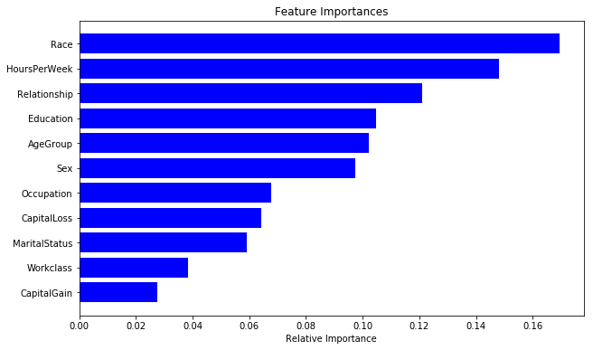

LightGBMSection titled LightGBM

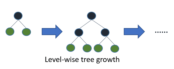
Similar to XGBoost, LightGBM is another optimized implementation of Gradient Boosting developed by Microsoft (similar to XGBoost available in Python, C++ and R). The main difference between LightGBM and other Gradient boosted trees (like XGBoost) implementations is in the way trees are grown. The details of this can be found on their features page. Briefly, LightGBM splits the tree leaf-wise with the best fit whereas other boosting algorithms split the tree depth-wise or level-wise. The two approaches can be best visualized in the following illustrations:

Level-wise Splits

Leaf-wise Splits

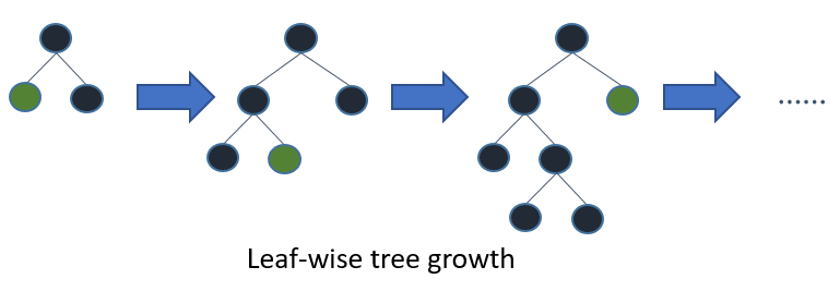
Leaf-wise splits lead to increase in complexity and may lead to over-fitting, and hence extra caution needs to be taken in tuning. Some of the biggest advantages of LightGBM over XGBoost is in terms of extremely fast training speed, lower memory usage, compatibility with large datasets and highly parallel computational support using threads, MPI and GPUs. LightGBM also has inbuilt support for categorical variables, unlike XGBoost, where one has to pre-process the data to convert all of the categorical features to integer ones using one-hot encoding or label encoding.

Since the trees are grown differently in LightGBM, its tuning procedure is quite different than XGBoost. Note that the latest version of XGBoost also provides a tree building strategy (depth-wise) which is quite similar to LightGBM.

All the parameters described above for XGBoost are also valid for LightGBM library. However, some parameters can have different names. Given the strategy of growing trees is different in LightGBM, an additional parameter needs to be tuned as well.

num_leaves: Maximum tree leaves for base learners. Note that since trees are grown depth-first, this parameters is independent of the max_depth parameter and has to be tuned independently. A typical value for starting should be much less than 2^{max _depth}.

When using the scikit-learn API of LightGBM, one should keep in mind that some of the parameter names are not standard ones (even though described in the API reference). In particular, I found that seed and nthreads as parameters, instead of random_state and n_jobs, respectively.

Let us tune a LightGBM model for the problem of Income prediction.

import lightgbm as lgb

params = {
    'n_estimators': 100,
    'num_leaves': 48,
    'max_depth': 6,
    'subsample': 0.75,
    'learning_rate': 0.1,
    'min_child_samples': 8,
    'seed': 32,
    'nthread': 8
}
lclf = lgb.LGBMClassifier(**params)

lclf.fit(x_train, y_train)
lclf.score(x_test, y_test)

This results in test accuracy of 86.8%.

Given this library also has many parameters, similar to XGBoost, we need to use a similar strategy of tuning in stages.

First we will fix learning rate to a reasonable value of 0.1 and number of estimators = 200, and tune only the major tree building parameters: max_depth, subsample, colsample_bytree and num_leaves. We will use the genetic algorithm to search for optimal values of these parameters.

ind_params = {
    'seed': 32,
    'n_estimators': 200,
    'learning_rate': 0.1,
    'nthread': 1
}
params = {
    'max_depth': (4, 6, 8),
    'subsample': (0.75, 0.8, 0.9, 1.0),
    'colsample_bytree': (0.75, 0.8, 0.9, 1.0),
    'num_leaves': (12, 16, 36, 48, 54, 60, 80, 100)
}

clf2 = EvolutionaryAlgorithmSearchCV(
        estimator=lgb.LGBMClassifier(**ind_params),
        params=params,
        scoring="accuracy",
        cv=5,
        verbose=1,
        population_size=50,
        gene_mutation_prob=0.10,
        gene_crossover_prob=0.5,
        tournament_size=5,
        generations_number=100,
        n_jobs=8
    )
clf2.fit(x_train, y_train)

This gives the following set of optimal parameters:

Best individual is: {'max_depth': 6, 'subsample': 1.0, 'colsample_bytree': 0.75, 'num_leaves': 54}
with fitness: 0.870888486225853

Now, we can use grid search to fine tune the search of number of leaves parameter.

ind_params = {
    'seed': 32,
    'n_estimators': 200,
    'learning_rate': 0.1,
    'nthread': 1,
    'max_depth': 6,
    'subsample': 1.0,
    'colsample_bytree': 0.75,
}
params = {
          'num_leaves': (48, 50, 52, 54, 56, 58, 60)
         }

clf2 = GridSearchCV(lgb.LGBMClassifier(**ind_params), params, cv=5, n_jobs=8, verbose=1)
clf2.fit(x_train, y_train)
print(clf2.best_params_)

Similar to XGBoost, LightGBM also provides a cv() method that can be used to find optimal value of number of estimators using early stopping strategy. Another strategy would be to search for this parameter as well. In the following, I want to use this grid search strategy to find best value of number of estimators, just to show how tedious this can be!

ind_params = {
    'seed': 32,
    'learning_rate': 0.1,
    'nthread': 1,
    'max_depth': 6,
    'subsample': 1.0,
    'colsample_bytree': 0.75,
    'num_leaves': 54
}
params = {'n_estimators': (200,300,400,800,1000)}

clf2 = GridSearchCV(lgb.LGBMClassifier(**ind_params), params, cv=5, n_jobs=8, verbose=1)
clf2.fit(x_train, y_train)
print(clf2.best_params_)

params = {'n_estimators': (250,275,300,320,340,360,380)}

clf2 = GridSearchCV(lgb.LGBMClassifier(**ind_params), params, cv=5, n_jobs=8, verbose=1)
clf2.fit(x_train, y_train)
print(clf2.best_params_)

params = {'n_estimators': (322,324,325,326,327,328,330,332,334,336,338)}

clf2 = GridSearchCV(lgb.LGBMClassifier(**ind_params), params, cv=5, n_jobs=8, verbose=1)
clf2.fit(x_train, y_train)
print(clf2.best_params_)

We find that the optimal value of n_estimators to be 327.

Now, we can use the similar strategy to find and fine-tune the best regularization parameters.

ind_params = {
    'seed': 32,
    'learning_rate': 0.1,
    'n_estimators': 327,
    'nthread': 1,
    'max_depth': 6,
    'subsample': 1.0,
    'colsample_bytree': 0.75,
    'num_leaves': 54
}

params = {'reg_alpha' : [0,0.1,0.5,1],'reg_lambda' : [1,2,3,4,6],}

clf2 = GridSearchCV(lgb.LGBMClassifier(**ind_params), params, cv=5, n_jobs=8, verbose=1)
clf2.fit(x_train, y_train)
print(clf2.best_params_)

params = {'reg_alpha' : [0.2,0.3,0.4,0.5,0.6,0.7,0.9],'reg_lambda' : [1.5,2,2.5],}
clf2 = GridSearchCV(lgb.LGBMClassifier(**ind_params), params, cv=5, n_jobs=8, verbose=1)
clf2.fit(x_train, y_train)
print(clf2.best_params_)

params = {'reg_alpha' : [0.55,0.58,0.6,0.62,0.65,0.68],'reg_lambda' : [1.1,1.2,1.3,1.4,1.5,1.6,1.7,1.8,1.9],}
clf2 = GridSearchCV(lgb.LGBMClassifier(**ind_params), params, cv=5, n_jobs=8, verbose=1)
clf2.fit(x_train, y_train)
print(clf2.best_params_)

params = {'reg_alpha' : [0.61,0.62,0.63,0.64],'reg_lambda' : [1.85,1.88,1.9,1.95,1.98],}
clf2 = GridSearchCV(lgb.LGBMClassifier(**ind_params), params, cv=5, n_jobs=8, verbose=1)
clf2.fit(x_train, y_train)
print(clf2.best_params_)

Finally, we can decrease the learning rate to 0.01 and find the optimal value of n_estimators.

ind_params = {
    'seed': 32,
    'learning_rate': 0.01,
    'nthread': 1,
    'max_depth': 6,
    'subsample': 1.0,
    'colsample_bytree': 0.75,
    'num_leaves': 54,
    'reg_alpha': 0.62,
    'reg_lambda': 1.9
}
params = {'n_estimators': (3270,3280,3300,3320,3340,3360,3380,3400)}

clf2 = GridSearchCV(lgb.LGBMClassifier(**ind_params), params, cv=5, n_jobs=8, verbose=1)
clf2.fit(x_train, y_train)
print(clf2.best_params_)

params = {'n_estimators': (3325,3330,3335,3340,3345,3350,3355)}

clf2 = GridSearchCV(lgb.LGBMClassifier(**ind_params), params, cv=5, n_jobs=8, verbose=1)
clf2.fit(x_train, y_train)
print(clf2.best_params_)

params = {'n_estimators': (3326,3327,3328,3329,3330,3331,3332,3333,3334)}

clf2 = GridSearchCV(lgb.LGBMClassifier(**ind_params), params, cv=5, n_jobs=8, verbose=1)
clf2.fit(x_train, y_train)
print(clf2.best_params_)

We find the optimal n_estimators to be equal to 3327 for a learning rate of 0.01. We can now built a final LightGBM model using these parameters and evaluate the test data.

ind_params = {
    'seed': 32,
    'learning_rate': 0.01,
    'n_estimators': 3327,
    'nthread': 8,
    'max_depth': 6,
    'subsample': 1.0,
    'colsample_bytree': 0.75,
    'num_leaves': 54,
    'reg_alpha': 0.62,
    'reg_lambda': 1.9
}
lclf = lgb.LGBMClassifier(**ind_params)
lclf.fit(x_train, y_train)
lclf.score(x_test, y_test)

We get a test accuracy of 87.01%. Similar to previous cases, we can again look at the accuracy of individual classes using the following confusion matrix plot:

y_pred = lclf.predict(x_test)
cfm = confusion_matrix(y_test, y_pred, labels=[0, 1])
plt.figure(figsize=(10,6))
plot_confusion_matrix(cfm, classes=["<=50K", ">50K"], normalize=True)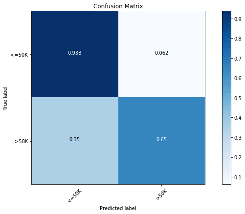

We find the results to be slightly better than XGBoost with 65% accuracy of the less abundant $>50K$ salary class. We can also look the importance of different features in this model:

importances = lclf.feature_importances_
indices = np.argsort(importances)
cols = [cols[x] for x in indices]
plt.figure(figsize=(10,6))
plt.title('Feature Importances')
plt.barh(range(len(indices)), importances[indices], color='b', align='center')
plt.yticks(range(len(indices)), cols)
plt.xlabel('Relative Importance')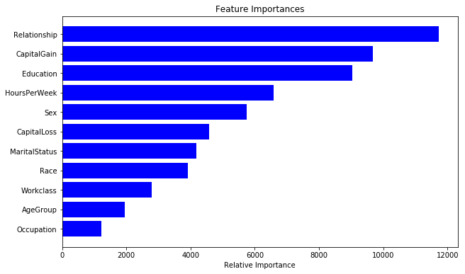

Concluding RemarksSection titled Concluding Remarks

XGBoost has been one of the most famous libraries used to win several machine learning competitions on Kaggle and similar sites. Slowly, LightGBM is also gaining traction due to its speed and parallelization capabilities. CatBoost is another boosting library from Yandex that has been shown to be quite efficient. I have used it personally yet though. If I find it to be worth making a move to, I will write about it in a future post.

Machine Learning, Algorithms