YOLO-v4 Object Detector

Object detection is useful for understanding what’s in an image, describing both what is in an image and where those objects are found. In general, there are two different approaches for this task:

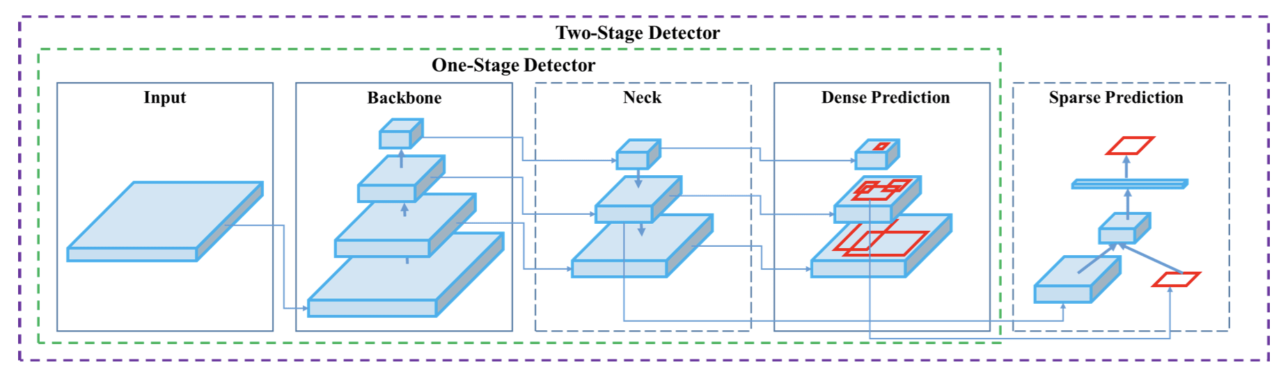
• Two-stage object-detection models – There are mainly two stages in these classification based algorithms. In the first stage, it will select a bunch of Region of Interest (ROI) in the image where the chances of objects are high. In the second stage, it will apply a Convolution Neural Network to these regions to detect the presence of an object. One of the problems with this method is, we have to execute the detector in each of the ROI, and that makes is slow and computationally expensive. Some common examples of these types of algorithms are Faster R-CNN, Mask R-CNN etc.

• One-stage object-detection models – In this class of algorithms, there is no selection of interesting ROI in the image, instead of that, it will predict the classes and bounding boxes for the entire image at once. This makes detection faster than two-stage algorithms. Some common examples of such algorithms are SSD, RetinaNet, FCOS, YOLO etc.

In this article, we are going to focus on a particular algorithm that belongs to the one-stage group. You only look once, or YOLO, is one of the faster object detection algorithms out there. Just recently, a new version of it YOLO v4 has been published. My goal here is to describe all the new updates made to this algorithm in this new version. The YOLO v4 paper focuses on developing an efficient, powerful, and high-accuracy object-detection model that can be quickly trained on standard GPU.

Object Detection Models: An OverviewSection titled Object Detection Models: An Overview

Essentially, the object-detection neural network is usually composed of three parts. The authors named them backbone, neck and head.

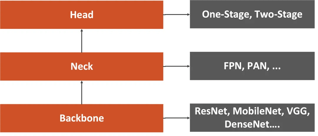
Backbone is usually deep architecture that was pre-trained on the ImageNet dataset without top layers. These are typically one of common CNN architectures like Resnet, VGGNet, Mobilenet etc. YOLO in particular uses a specialized version of backbone called ‘Darknet’.

Neck is usually composed of several layers whose goal is to collect feature maps from different stages. Common examples of “neck” are: Feature Pyramid Network (FPN), PAN, SPP, ASPP etc.

Head is a part of the object detection model that is used for the prediction of custom classes and drawing bounding boxes around objects. Based on the type of the head, we can distinguish two types of object-detection models described above. These layers can also be described in terms of dense predictors (one-stage detectors) or sparse predictors (two-stage detectors).

YOLO V3: An OverviewSection titled YOLO V3: An Overview

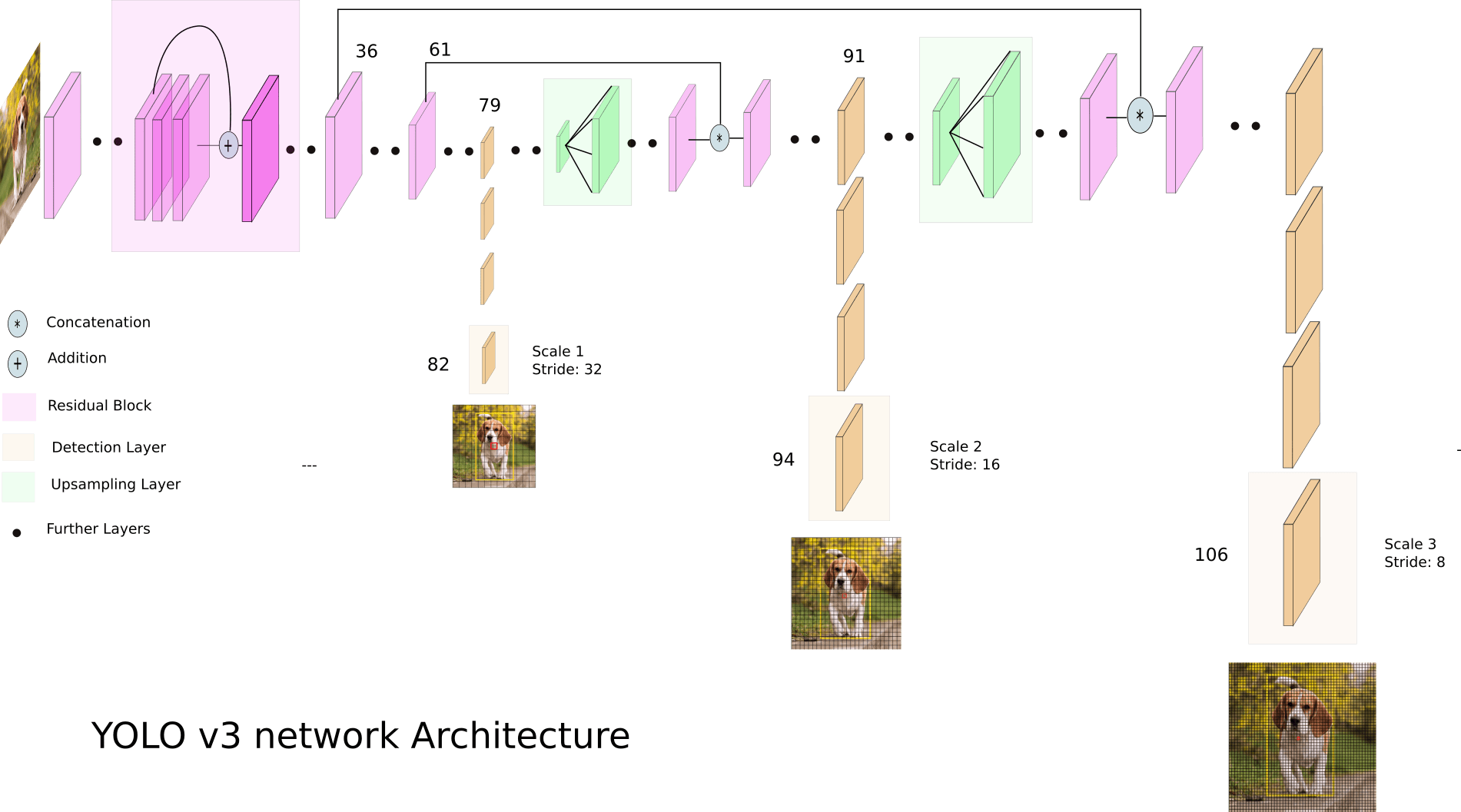
“Backbone” of YOLO v3 is a 53-conv layer network called Darknet-53. You can view of this as a resnet-like architecture. For the “Neck”, three different scales are used and three different scales are combined via upsampling and concatenation. See the complete network diagram below for details. Finally, the “Head” is a series of conv layers for dense predictions of box regressions and classification scores.

Bounding Box PredictionsSection titled Bounding Box Predictions

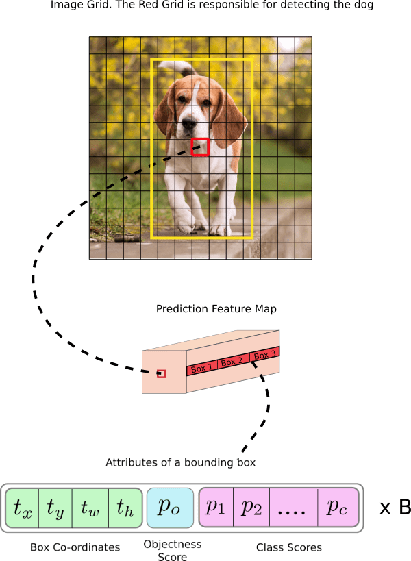
The most salient feature of v3 is that it makes detections at three different scales. YOLO is a fully convolutional network and its eventual output is generated by applying a 1 x 1 kernel on a feature map. In YOLO v3, the detection is done by applying 1 x 1 detection kernels on feature maps of three different sizes at three different places in the network.

The shape of the detection kernel is 1 x 1 x (B x (5 + C) ). Here B is the number of bounding boxes a cell on the feature map can predict, “5” is for the 4 bounding box attributes and one object confidence, and C is the number of classes. In YOLO v3 trained on COCO, B = 3 and C = 80, so the kernel size is 1 x 1 x 255. The feature map produced by this kernel has identical height and width of the previous feature map, and has detection attributes along the depth as described above.

The stride of the network, or a layer is defined as the ratio by which it downsamples the input. In the following examples, I will assume we have an input image of size 416 x 416. YOLO v3 makes prediction at three scales, which are precisely given by downsampling the dimensions of the input image by 32, 16 and 8 respectively.

The first detection is made by the 82nd layer. For the first 81 layers, the image is down sampled by the network, such that the 81st layer has a stride of 32. If we have an image of 416 x 416, the resultant feature map would be of size 13 x 13. One detection is made here using the 1 x 1 detection kernel, giving us a detection feature map of 13 x 13 x 255.

Then, the feature map from layer 79 is subjected to a few convolutional layers before being up sampled by 2x to dimensions of 26 x 26. This feature map is then depth concatenated with the feature map from layer 61. Then the combined feature maps is again subjected a few 1 x 1 convolutional layers to fuse the features from the earlier layer (61). Then, the second detection is made by the 94th layer, yielding a detection feature map of 26 x 26 x 255.

A similar procedure is followed again, where the feature map from layer 91 is subjected to few convolutional layers before being depth concatenated with a feature map from layer 36. Like before, a few 1 x 1 convolutional layers follow to fuse the information from the previous layer (36). We make the final detection of the 3 at 106th layer, yielding feature map of size 52 x 52 x 255.

YOLO v3, in total uses 9 anchor boxes. Three for each scale. Authors use k-means clustering to determine our bounding box priors. In total they choose 9 clusters and 3 scales arbitrarily and then divide up the clusters evenly across scales - arrange the anchors is descending order of a dimension. Assign the three biggest anchors for the first scale , the next three for the second scale, and the last three for the third. Hence, at each grid point, YOLO v3 predicts 3 boxes at each of the scales, thus predicting a total of 13x13x3 + 26x26x3 + 52x52x3 = 10647 boxes for each image!

Loss FunctionSection titled Loss Function

YOLOv3 predicts an objectness score for each bounding box using logistic regression. This should be 1 if the bounding box prior overlaps a ground truth object by more than any other bounding box prior. If the bounding box prior is not the best but does overlap a ground truth object by more than some threshold (0.5) we ignore the prediction. It assigns one bounding box prior for each ground truth object. If a bounding box prior is not assigned to a ground truth object it incurs no loss for coordinate or class predictions, only objectness.

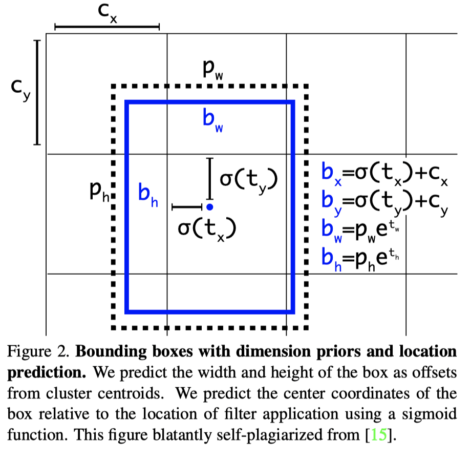
The complete loss terms related to localization for YOLOv3 can be seen in the figure above. In summary, The network predicts 4 coordinates for each bounding box, $t_x$ , $t_y$ , $t_w$ , $t_h$. If the cell is offset from the top left corner of the image by ($c_x$ , $c_y$) and the bounding box prior has width and height $p_w$ , $p_h$, then the predictions correspond to:

The localization loss is the sum of squared error loss on these terms. If the ground truth for some coordinate prediction is $\hat{t}_*$ , then gradient is the ground truth value (computed from the ground truth box) minus our prediction: $\hat{t}_* - t_*$. This ground truth value can be easily computed by inverting the equations above.

YOLO V4 ModificationsSection titled YOLO V4 Modifications

Authors introduce two terms Bag of freebies (BOF) and Bag of specials (BOS). Bag of freebies refers to the methods that affect training strategy. One such method is data augmentation, which is used to increase the variability of the input images and make the model has increased robustness. Other methods that could be considered as Bag of freebies are random erase, CutOut, grid mask, DropOut, DropConnect, etc. All these methods temper with the input images and/or feature maps and remove bias from input data. Another set of bag of freebies could be related to loss terms associated with bounding boxes - instead of traditional mean squared loss, using a loss term that is associated with the IoU wrt ground truth boxes.

Bag of specials are post-processing modules and methods that do increase the inference cost but improve the accuracy of object detection as well. These can be any methods enhancing certain features of a model. For example, that can be enlarging receptive field, introducing attention mechanism, or strengthening feature integration capability, etc.

Based on all of these, the architecture of YOLOv4 consists of the following updates:

• Backbone: CSPDarknet53 – Cross Stage Partial Network minimizing required heavy inference computations from the network architecture perspective. CSPDarknet53 is an updated version of the Darknet-53 network based on concepts from CSPNet. Main advantages of using CSPNet comes from use of partial blocks and transition layers that increase gradient path, balance computation of each layer and reduce memory traffic.

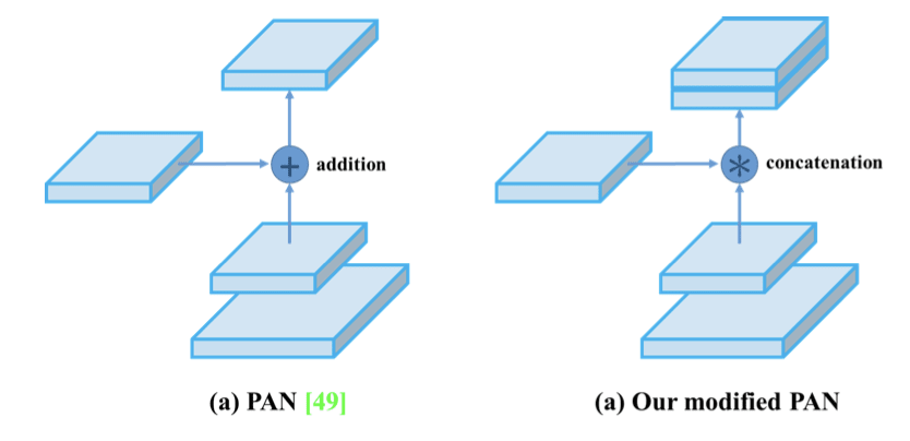
• Neck: Spatial Pyramid Pooling (SPP) added at the end of the backbone so object-detector can receive images of arbitrary size/scale. Instead of FPN like aggregation used in YOLOv3, Path Aggregation Network (PANet) is used in the neck for boosting information flow. PANet adds an additional bottom-up pathway of information flow. Authors have further tweaked the regular PANet module, where they use “concatenation” instead of “addition” used in the original module.

• Head: Same as YOLOv3.

Bag of Freebies (BoF) for backboneSection titled Bag of Freebies (BoF) for backbone

• CutMix and
• Mosaic data augmentation,
• DropBlock regularization,
• Class label smoothing.

Authors propose a new type of data augmentation method called Mosaic that mixes 4 training images. Thus 4 different contexts are mixed, while CutMix mixes only 2 input images. This allows detection of objects outside their normal context. In addition, batch normalization calculates activation statistics from 4 different images on each layer. This significantly reduces the need for a large mini-batch size.

DropBlock regularization

In Fully-connected layers, we can apply dropoff to force the model to learn from a variety of features instead of being too confident on a few. However, this may not work for convolution layers. Neighboring positions are highly correlated. So even some of the pixels are dropped (the middle diagram below), the spatial information remains detectable. DropBlock regularization builds on a similar concept that works on convolution layers.

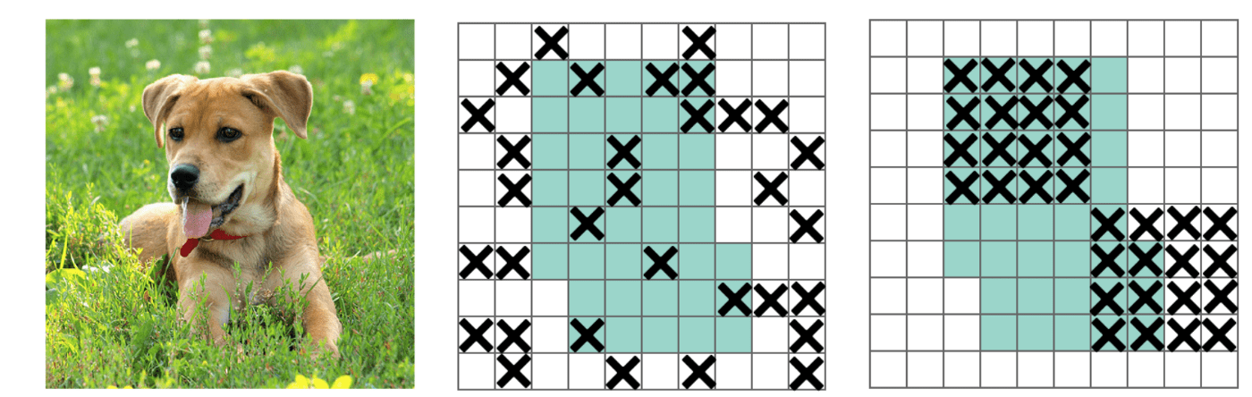
Instead of dropping individual pixels, a block of block_size × block_size of pixels is dropped.

Class label smoothing acts as a regularizer, a typical formulation for it can be:

where $C$ is the number of label classes, and $\alpha$ is a hyperparameter that determines the amount of smoothing.

Bag of Specials (BoS) for backboneSection titled Bag of Specials (BoS) for backbone

• Mish activation,
• Cross-stage partial connections (CSP),
• Multi input weighted residual connections (MiWRC)

Multi-input weighted residual connections (MiWRC)

For the past few years, researchers have paid a lot of attention to what feature maps will be fed into a layer. Sometimes, we break away from the tradition that only the previous layer is used.

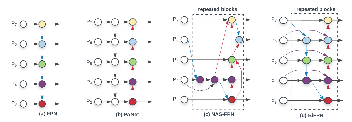
How layers are connected becomes more important now, in particular for object detectors. We have discussed FPN and PAN so far as examples. The diagram below shows another neck design called BiFPN that has better accuracy and efficiency trade-offs according to the BiFPN paper.

EfficientDet is considered as one of the most accurate object detectors. Hence, some of its features can be used to improve YOLO V4. EfficientDet uses the EfficientNet as the backbone feature extractor and BiFPN as the neck.

Based on the observation, as noted in the EfficientDet paper, different input features are at different resolutions and it contributes to the output feature unequally. YOLOv4 captures this aspect of EfficientDet by using Multi-input weighted residual connections.

Bag of Freebies (BoF) for detectorSection titled Bag of Freebies (BoF) for detector

• CIoU-loss
• Cross mini-batch Normalization (cmBN)
• DropBlock regularization
• Mosaic data augmentation,
• Self-Adversarial Training,
• Eliminate grid sensitivity,
• Using multiple anchors for single ground truth,
• Cosine annealing scheduler,
• Optimal hyperparameters,
• Random training shapes

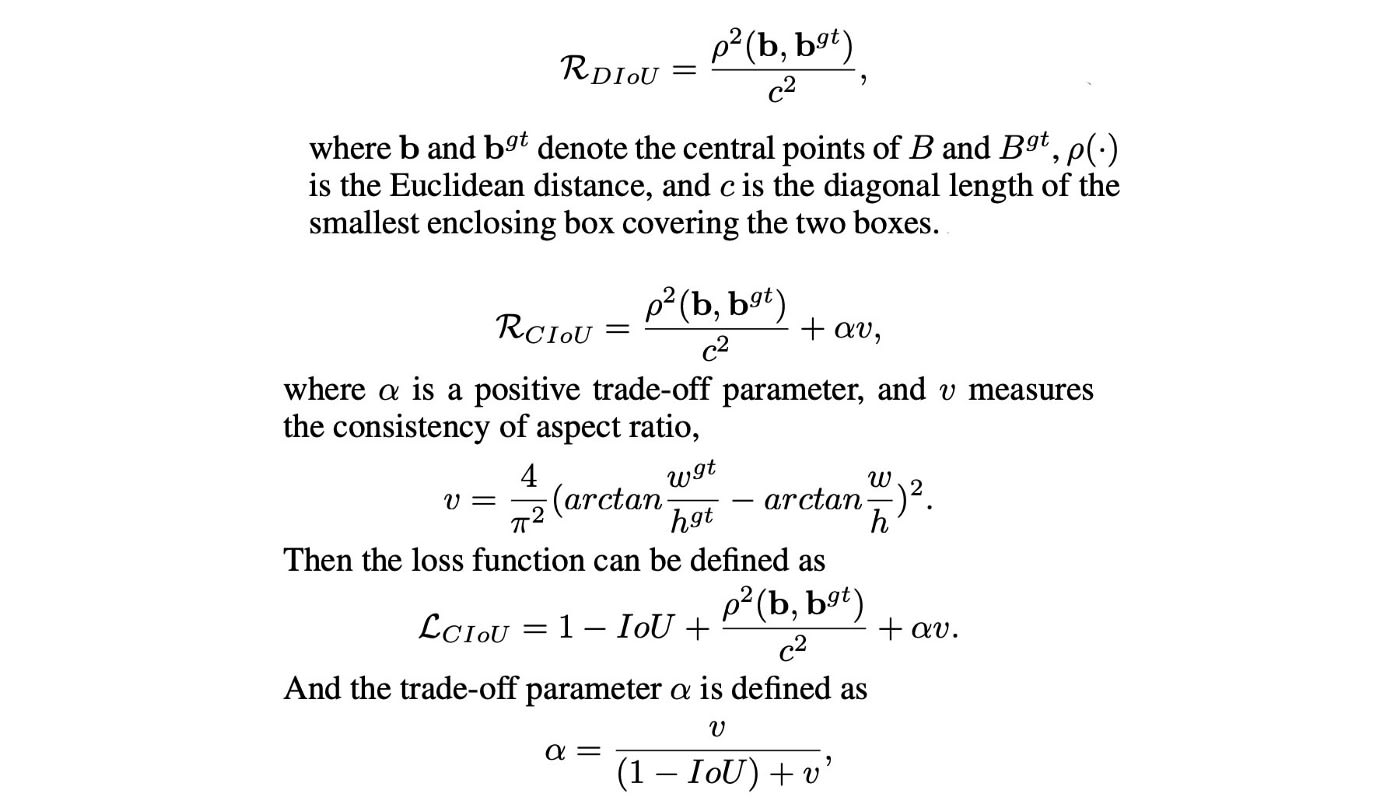
CIoU-loss

A loss function gives us signals on how to adjust weights to reduce cost. So in situations where we make wrong predictions, we expect it to give us direction on where to move. But this is not happening when IoU is used and the ground truth box and the prediction do not overlap. Consider two predictions that both do not overlap with the ground truth, the IoU loss function, as described in equations below, cannot tell which one is better even one may be closer to the ground truth than the other.

Where $B$ is the bounding box and $B^{gt}$ is the ground truth box.

Generalized IoU (GIoU) fixes this by refining the loss as:

where $C$ is the smallest box covering $B$ and $B^{gt}$.

But this loss function tends to expand the prediction bounding box first until it is overlapped with the ground truth. Then it shrinks to increase IoU. This process requires more iterations than theoretically needed.

First, Distance-IoU Loss (DIoU) was introduced as:

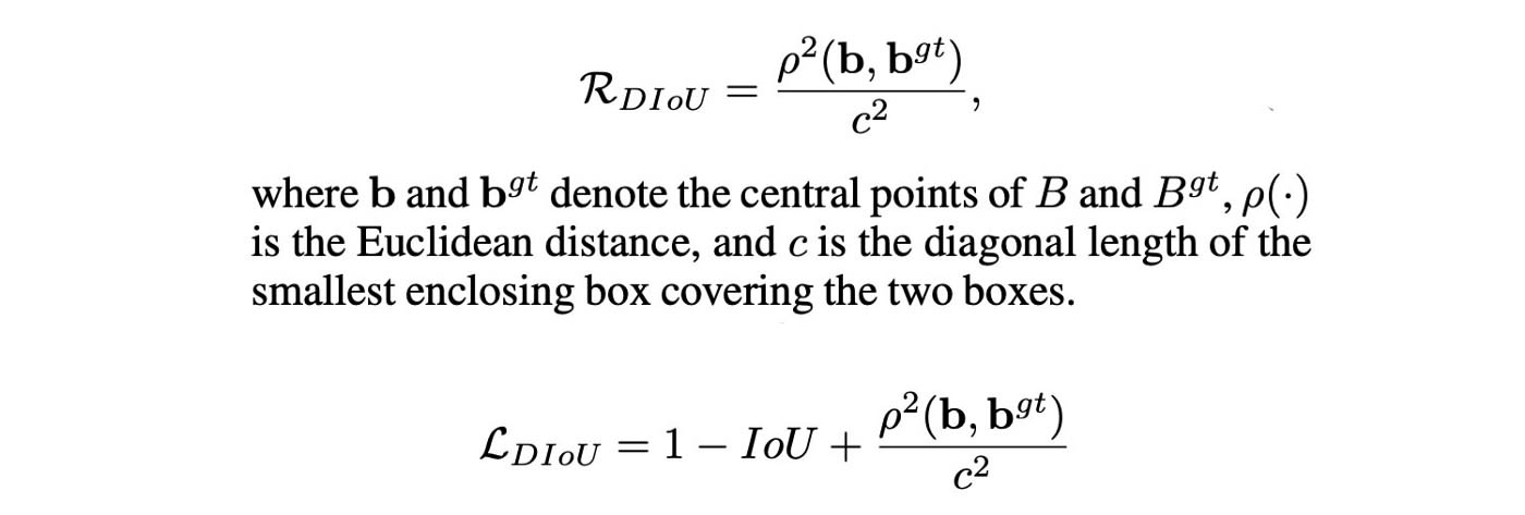
It introduces a new goal to reduce the central points separation between the two boxes.

Finally, Complete IoU Loss (CIoU) was introduced to increase the overlapping area of the ground truth box and the predicted box, minimize their central point distance, and maintain the consistency of the boxes’ aspect ratio.

Cross mini-batch Normalization (cmBN)

The original Batch normalization collects the mean and the variance of the samples within a mini-batch to whiten the layer input. However, if the mini-batch size is small, these estimations will be noisy. One solution is to estimate them among many mini-batches. However, as weights are changing in each iteration, the statistics collected under those weights may become inaccurate under the new weight. A naive average will be wrong. Fortunately, weights change gradually. In Cross-Iteration Batch Normalization (CBM), it estimates those statistics from k previous iterations with the adjustment, as described below:

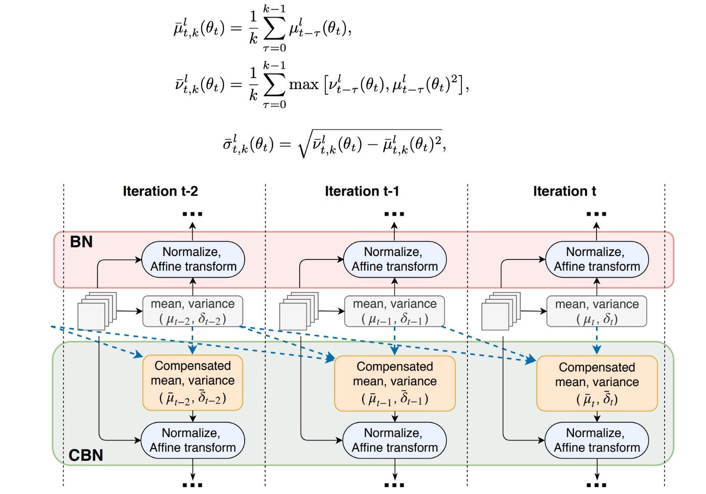
CmBN is a modified option that collects statistics only between mini-batches within a single batch.

Self-Adversarial Training (SAT)

SAT is a data augmentation technique. First, it performs a forward pass on a training sample. Traditionally, in the backpropagation, we adjust the model weights to improve the detector in detecting objects in this image. Here, it goes in the opposite direction. It changes the image such that it can degrade the detector performance the most. i.e. it creates an adversarial attack targeted for the current model even though the new image may look visually the same. Next, the model is trained with this new image with the original bounding box and class label. This helps to generalize the model and to reduce overfitting.

Eliminate grid sensitivity

In YOLO, the bounding box $b$ is computed as:

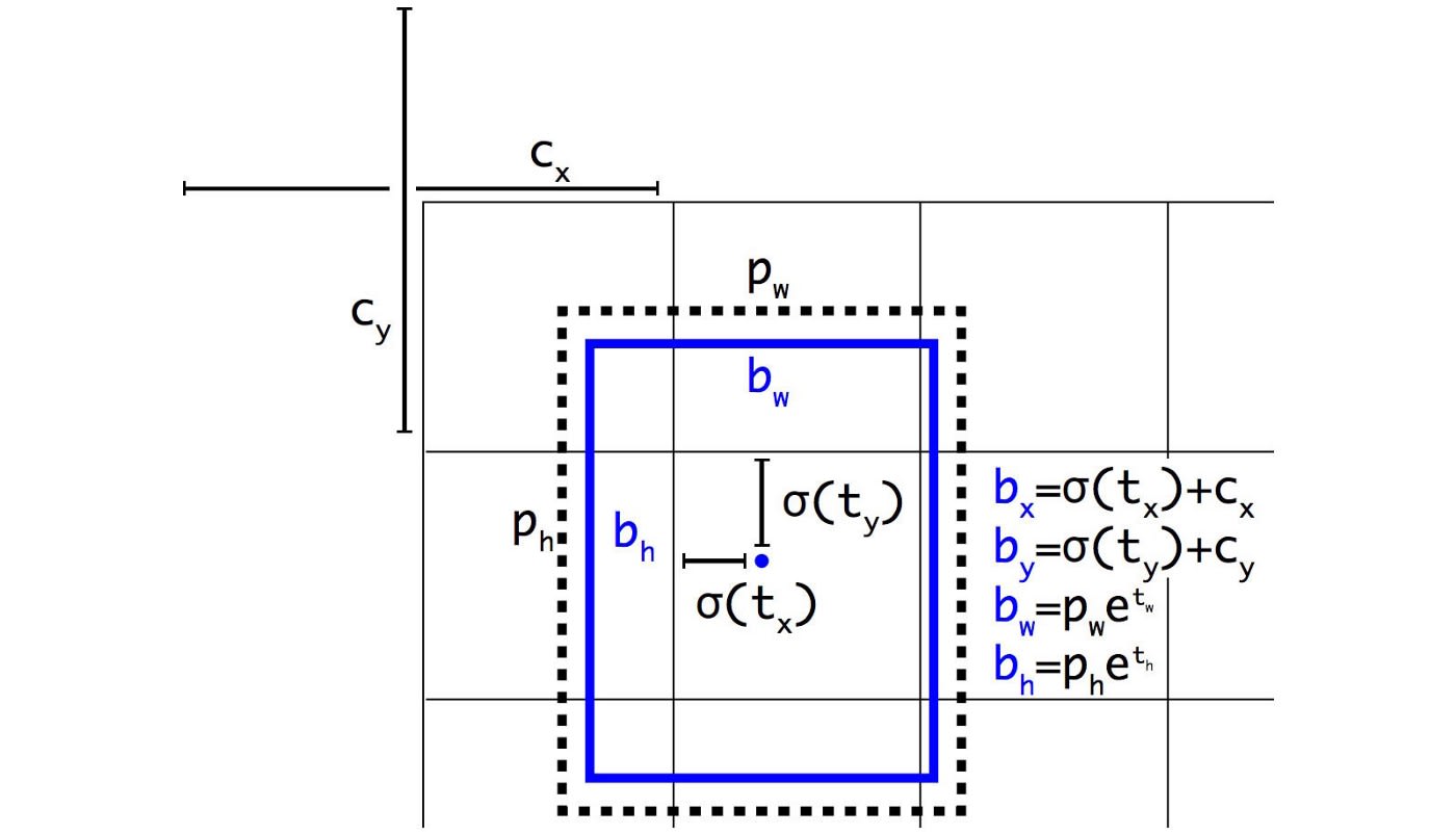
For the case $b_x = c_x$ and $b_x = c_x + 1$, we need $t_x$ to have a huge negative and positive value, respectively. But we can multiply $\sigma$ with a scaling factor (> 1.0) to make this happen quite easily.

Multiple anchors for a single ground truth

Use multiple anchors for a single ground truth if IoU (ground truth, anchor) > IoU threshold. I am not convinced though how this helps!

Bag of Specials (BoS) for detectorSection titled Bag of Specials (BoS) for detector

• Mish activation
• SPP-block,
• Modified SAM-block,
• Modified PAN path-aggregation block,
• DIoU-NMS

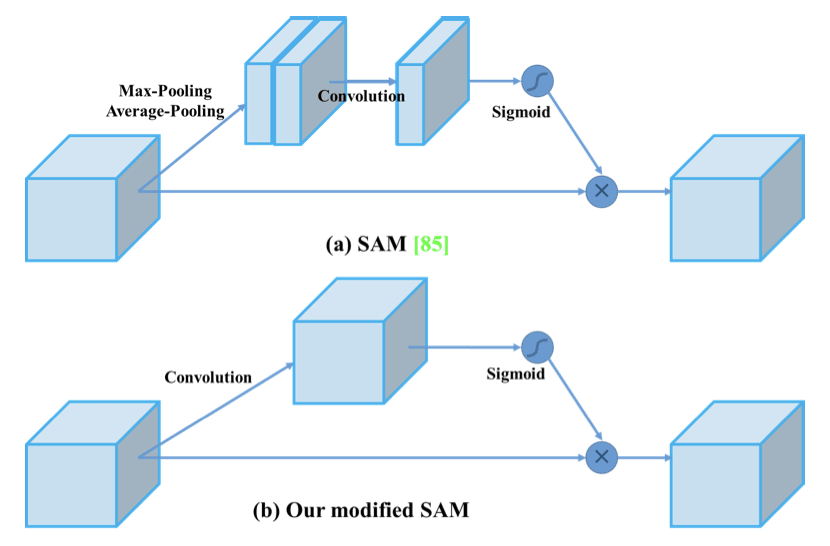
Spatial Attention Module (SAM)

Attention has widely adopted in DL designs. In SAM, maximum pool and average pool are applied separately to input feature maps to create two sets of feature maps. The results are feed into a convolution layer followed by a sigmoid function to create spatial attention.

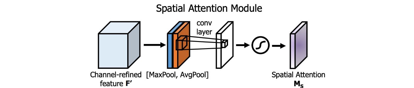
This spatial attention mask is applied to the input feature to output the refined feature maps.

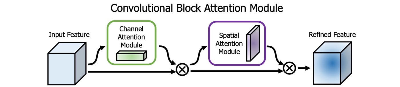
In YOLOv4, a modified SAM is used without applying the maximum and average pooling.

In YOLOv4, the FPN concept is gradually implemented/replaced with the modified SPP, PAN, and SAM.

DIoU-NMS

NMS filters out other bounding boxes that predict the same object and retains one with the highest confidence.

DIoU (See Equations Above) is employed as a factor in non-maximum suppression (NMS). This method takes IoU and the distance between the central points of two bounding boxes when suppressing redundant boxes. This makes it more robust for the cases with occlusions.

Results SummarySection titled Results Summary

A comparison of results for YOLOv4 with other object detection models on MS COCO dataset with Maxell GPU is shown in the table below. In particular here we are looking only for speed (FPS - frames per second), and accuracy (AP - average pecision and AP_small - average precision for small objects only).

Comparing results with other detectors is pretty impressive! They outperform in terms of both speed and average precision scores.

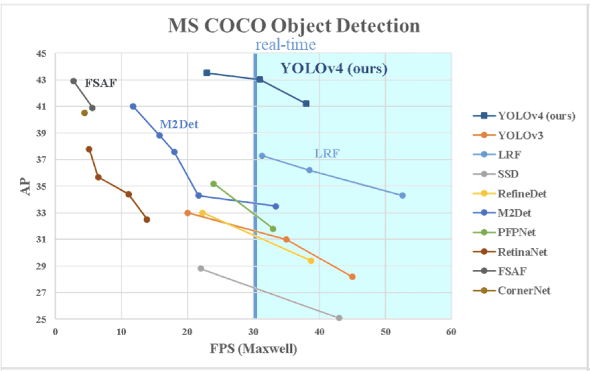
A not so thorough analysis of effects of different modifications can be found in the paper.