Evaluating Comet for Managing Pytorch Based Deep Learning Experiments

Managing multiple research experiments at a time can be overwhelming. The same applies to deep learning research as well. Beyond the usual challenges in software development, machine learning developers face new challenges - experiment management (tracking which parameters, code, and data went into a result) and reproducibility (running the same code and environment later)!

Being an active researcher in deep learning, I run multiple experiments every day for exploring different ideas. Managing this very iterative task is very crucial in obtaining good models. In this article, I will describe my setup for using Pytorch and evaluate comet.ml for the management of experiments.

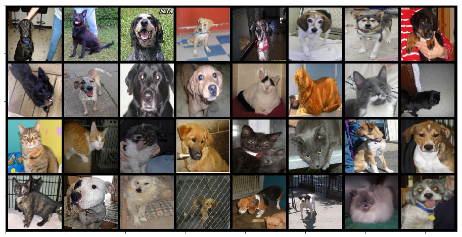
I am going to consider the problem of classification of cats and dogs. You can download the data from here. This has 12500 images each of cats and dogs. First thing, we will do is to clean up the data - remove non-image files, convert images to standard 3 channel RGB PNG images and remove any corrupt image files. Additionally, we also want to divide our data into training and testing sets. For this problem, I decided to put 10,000 images each of cats and dogs in training and remaining 2500 images each of cats and dogs in the testing data set. I use the following python code to achieve this:

import glob
import random
from PIL import Image

cats = glob.glob('~/Downloads/PetImages/Cat/*.*')
random.shuffle(cats)

dogs = glob.glob('~/Downloads/PetImages/Dog/*.*')
random.shuffle(dogs)

train_cats, test_cats = cats[:10000], cats[10000:]
train_dogs, test_dogs = dogs[:10000], dogs[10000:]

def write_data(data, mode, animal):
    for d in data:
        d_fname_base = d.split('/')[-1].split('.')[0]
        d_fname = f'/data/data/cats-and-dogs/{mode}/{animal}/{d_fname_base}.png'
        try:
            im = Image.open(d)
        except IOError:
            print(f'skipping image {d}')
            continue
        rgb_im = im.convert('RGB')
        rgb_im.save(d_fname)

write_data(train_cats, 'train', 'cat')
write_data(test_cats, 'test', 'cat')

write_data(train_dogs, 'train', 'dog')
write_data(test_dogs, 'test', 'dog')

Now that we have the data, We can take a look into the code format that I use for training pytorch models. Pytorch is very research friendly framework giving you a flexible framework to code new research ideas pretty quickly. However, it lacks any high level API like Keras. I use this pretty handy template to code my models, which I started from this github repository. The main idea in this template is about segregating logic for models, data loaders, training process and its different components. You can clone my code from this github repository. This repository also has an “mnist” branch to get you started quickly. The file structure of the codebase is as follows:

.
├── LICENSE
├── README.md
├── base
│   ├── __init__.py
│   ├── base_data_loader.py
│   ├── base_model.py
│   └── base_trainer.py
├── config.json
├── data
├── data_loader
│   └── data_loaders.py
├── model
│   ├── loss.py
│   ├── metric.py
│   └── model.py
├── saved
├── test.py
├── train.py
├── trainer
│   ├── __init__.py
│   └── trainer.py
└── utils
    ├── __init__.py
    ├── logger.py
    └── util.py

The original codebase for this template uses tensorboard to log experiments. However, I find tensorboard to be very rudimentary for the purpose of tracking of experiments.

During my search for tools for managing deep learning experiments, I came across comet.ml. It has some interesting features:

• Tracking of code, git sha key (if run from a git repository)
• Tracking of hyperparameters / config file
• Graph definition visualization per experiment
• Tabular view of metrics
• Plots of metrics and losses in both training and testing modes
• comparison of two experiments
• grouping experiments across projects
• steps to replicate an experiment
• logging images etc. (model outputs) for an experiment

These features were interesting enough for me to start evaluating this. To get started, I had to open an account with comet.ml. One can use his/her github credentials for a quick setup. Once inside the account, you can get your API_KEY from the settings. I found the best place to save this is in a file named .comet.config in the home directory.

# cat ~/.comet.config

[comet]
api_key=YOUR-API-KEY

I have set up automatic comet tracking of experiments in my pytorch template library. It can be enabled by setting comet parameter in the config.json file to true. The experiment is saved under the project whose name is based on the name parameter in the config.json file.

Coming back to the cats vs dogs classification problem, I explored it using transfer learning. Specifically, I have used an imagenet pre-trained VGG16 model with Batch Norm (available in the torchvision.models module).

I performed the following set of experiments to track and compare them in comet:

• Use features from pretrained VGG16-BN model and add two fully connected layers with dropout. Use SGD optimizer with a learning rate of 0.001.
• Same as above with a higher learning rate of 0.004.
• Same as above with Adam optimizer (same two learning rates).

class VGG16BN(BaseModel):
    def __init__(self, num_classes=2):
        super().__init__()
        self.features = vgg16_bn(pretrained=True).features
        self.avgpool = nn.AdaptiveAvgPool2d(7)
        self.classifier = nn.Sequential(
            nn.Linear(512 * 7 * 7, 128), nn.ReLU(True), nn.Dropout(), nn.Linear(128, num_classes)
        )
        # freeze all layers of feature extractor
        for param in self.features.parameters():
            param.requires_grad = False
        self._initialize_classifier_weights()

    def _initialize_classifier_weights(self):
        for m in self.classifier.modules():
            if isinstance(m, nn.Conv2d):
                nn.init.kaiming_normal_(m.weight, mode='fan_out', nonlinearity='relu')
                if m.bias is not None:
                    nn.init.constant_(m.bias, 0)
            elif isinstance(m, nn.BatchNorm2d):
                nn.init.constant_(m.weight, 1)
                nn.init.constant_(m.bias, 0)
            elif isinstance(m, nn.Linear):
                nn.init.normal_(m.weight, 0, 0.01)
                nn.init.constant_(m.bias, 0)

    def forward(self, x):
        x = self.features(x)
        x = self.avgpool(x)
        x = x.view(x.size(0), -1)
        return self.classifier(x)

For the training data, I do the following set of transforms on the data:

• Random Crop and Resize: A crop of random size (default: of 0.08 to 1.0) of the original size and a random aspect ratio (default: of 3/4 to 4/3) of the original aspect ratio is made. This crop is finally resized to 224x224.
• Random Horizontal Flip: Horizontally flip the given image randomly with a probability of 0.5.

For testing data, I only resize the images to 224x224 size. In both cases, images are standardized by the following mean and variance values (values used in Imagenet).

normalize = transforms.Normalize(mean=[0.485, 0.456, 0.406], std=[0.229, 0.224, 0.225])

I first ran all 4 experiments (SGD and Adam optimizers with learning rates of 0.001 and 0.004). As you can see in the screen shots below, it is quite handy to view progress of individual experiments:

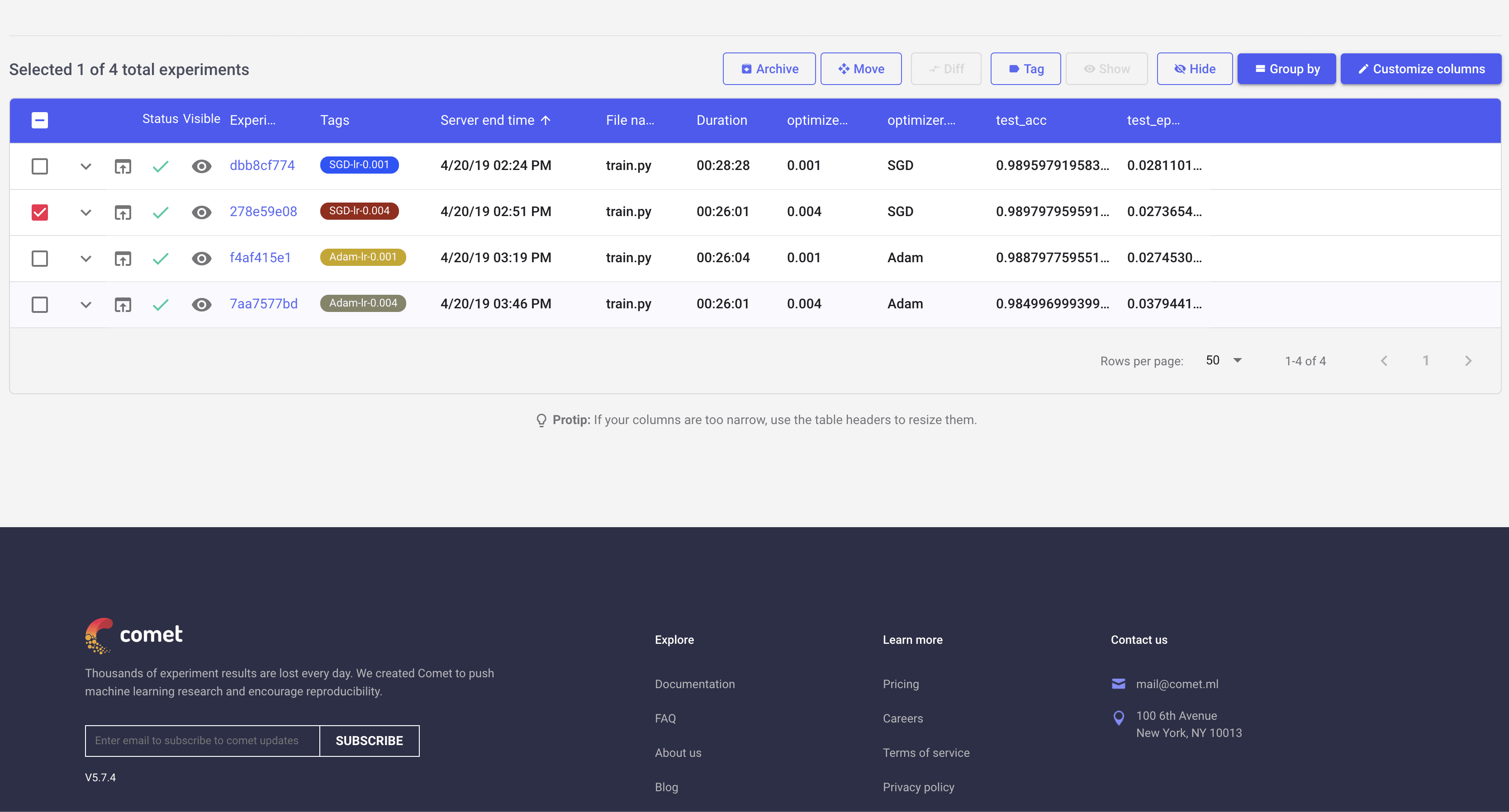
This list view can be customized to show different parameters and metrics in the table. Here I have added few of those to easily distingush different experiments.

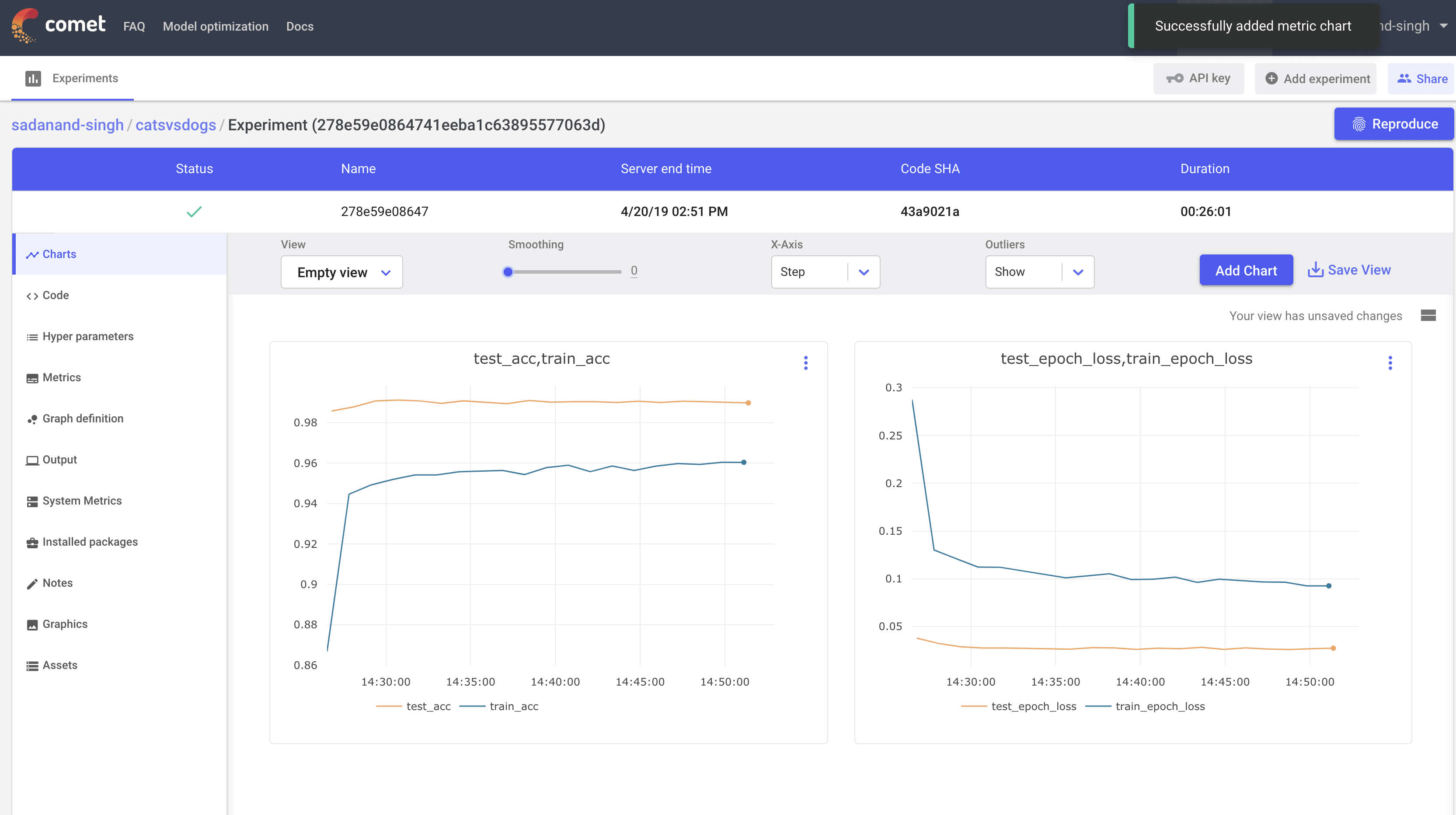
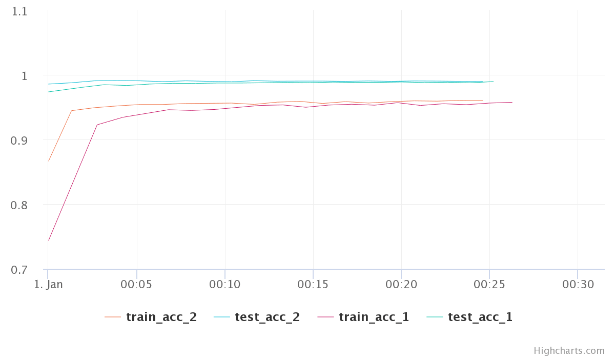
Let us first take a look at the best performing model (SGD with a learning rate of 0.004). Clicking this particular experiment, takes us into its expanded view, where we can look at different charts, a tabular view with min/max of different metrics, code, parameters etc. By default, you get individual plots for losses and metric for train and test modes. However, you can create your own set of plots. Here, I created plots to compare test/train accuracy and losses.

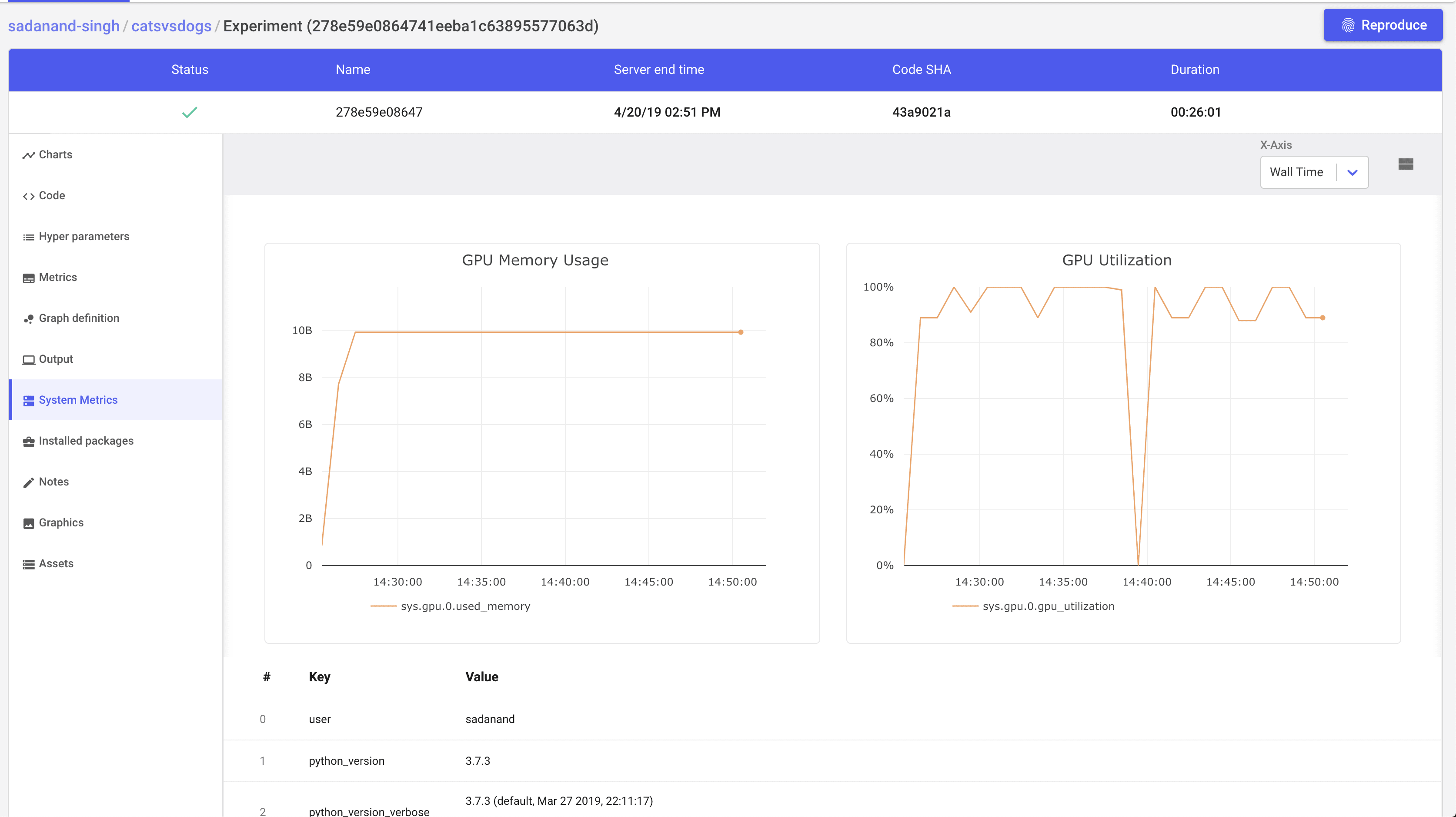
Additionally, we get other handy information like list of hyper parameters, gpu utilization and a tabular view of metrics.

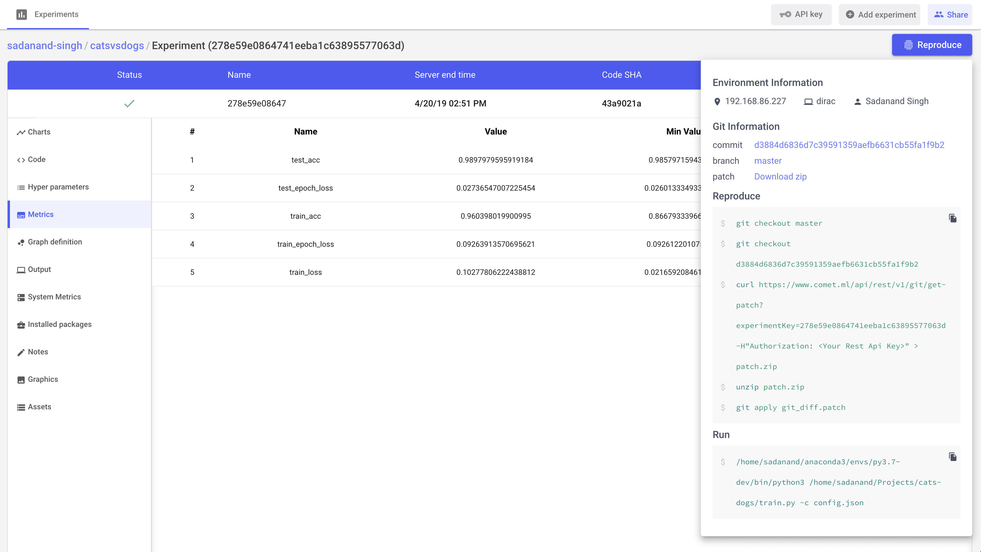
A really cool feature that I really like, is to get steps to reproduce to the results for a given experiment.

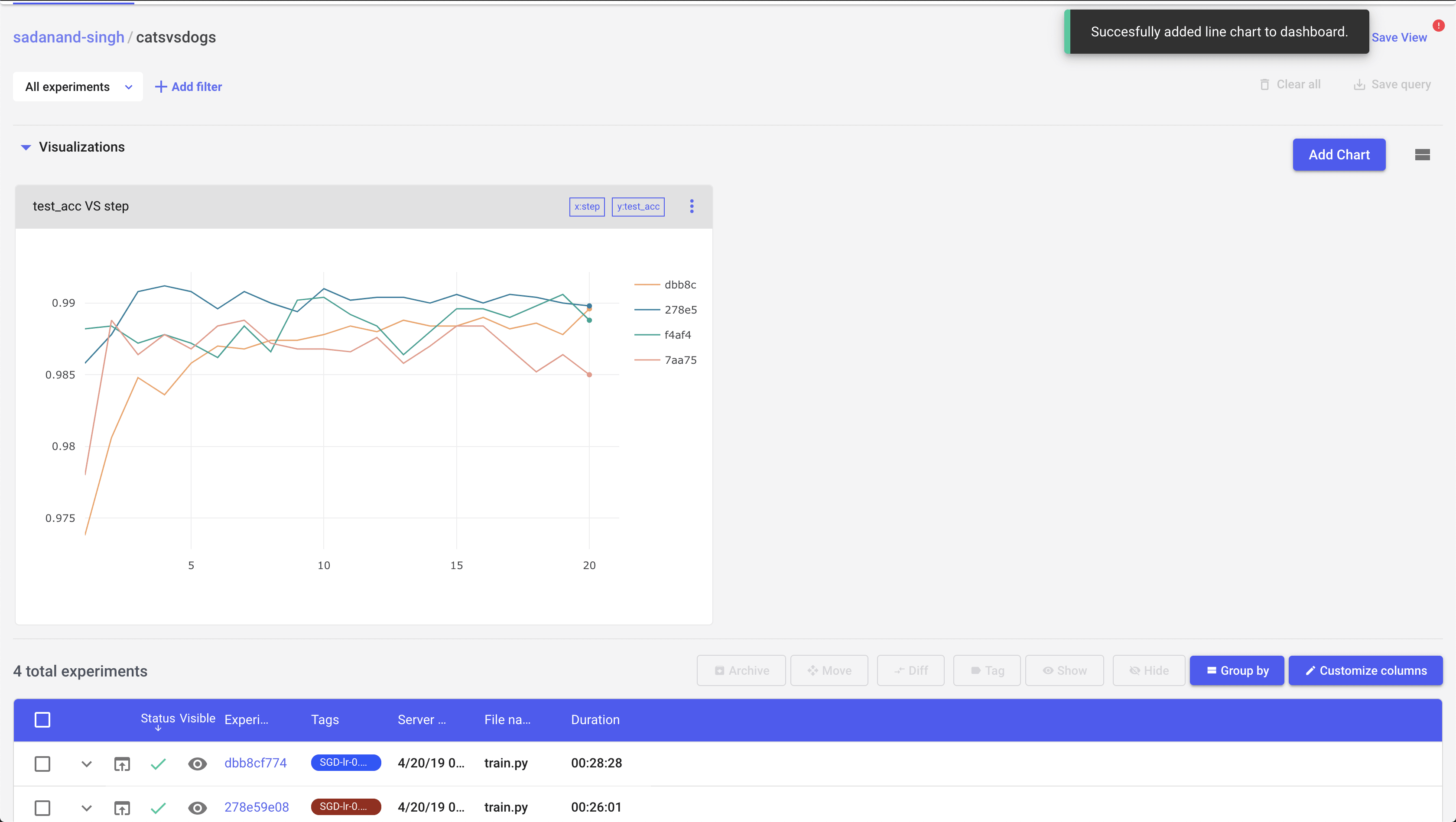
So far things were looking good. Now, I wanted to compare these experiments graphically. On the page where you get a list view of experiments, there is an option to plot some metrics as a function of experiments. It’s pretty easy to add a comparison chart for some given metric and compare different experiments pretty quickly:

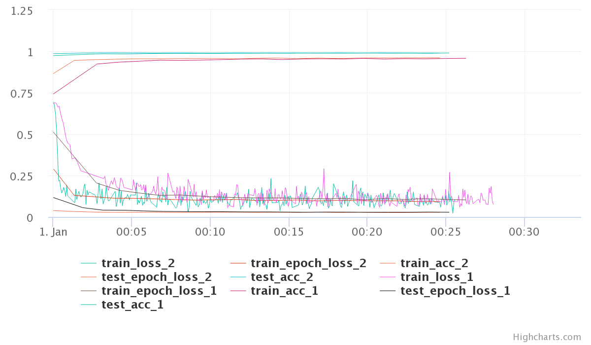
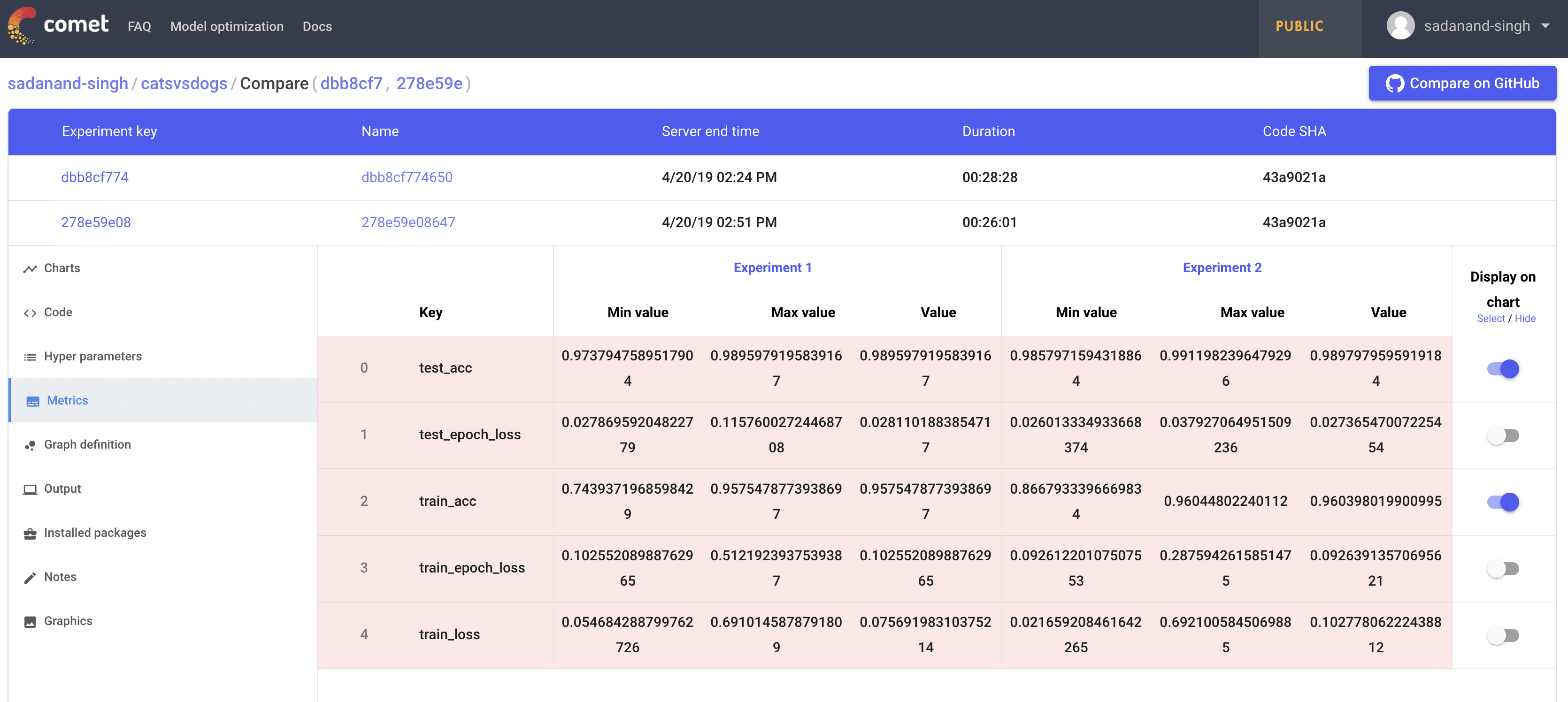
Moving on, Any two experiments can be selected to get a diff between them. Selecting any two experiments, and pressing the “Diff” button takes you to a comparison view of two experiments. I found this to be little bit of a mixed experience. You can see individual experiment charts as well as both of them on single chart. However, these charts are extremely basic.

The chart here is very crowded and the colors are very unreadable. The worst part is that you have no control over the choice of colors. Even for this simple toy example with just a few metrics the above plots is very crowded. Different metrics can be compared in a table as well. Oddly, you can control here which ones get plotted in the graph.

However, even with limiting what graphs we see for the comparison, the graphs are not usable. I was hoping to get more control over plotting, may be even on-demand plotting.

Considering the most of the real life examples are much more complex than a simple cat vs dog model, these comparison graphs and over all process have to be modified and tuned heavily to make it work for real life deep learning projects. I also looked briefly at uploading of images and assets, however, I found it to be not too friendly to use.

Overall, I think comet is a good step towards democratization of deep learning. It is still in early stage to be completely usable in all sorts of projects. One aspect that I personally do not like about this is how all your data ends up going to comet servers. Because of this, I have started to look into tools that work locally. Please share your thoughts and suggestion about this if it interests you on twitter.