An Overview of Linear Regression Models

Modeling the relationship between a scalar response (or dependent variable) and one or more explanatory variables (or independent variables) is commonly referred as a regression problem. The simplest model of such a relationship can be described by a linear function - referred as linear regression.

Table of ContentsSection titled Table of Contents

Mathematical formulationsSection titled Mathematical formulations

Linear Regression represents a linear relationship between the input variables ($X$) and single output variable($y$). When the input ($X$) is a single variable, this model is called Simple Linear Regression and when there are multiple input variables ($X$), it is called Multiple Linear Regression. Mathematically, a simple linear regression model can be represented as,

For $n$ data points, we can write these equations in matrix form as,

For the general case of multi-dimensional input variable, $X \equiv$ $x_{i1}, x_{i2}, \ldots x_{im}$, we can write the above matrix equation as,

In matrix notation, this can be written as,

In terms of a regression problem, given the data $\mathbf{X}$ and the true response $y$, we want to estimate the weights vector $w$, such that the predicted response $\hat{y} = \mathbf{X}w$ is as close as possible to $y$.

The most common way to define and get the closeness of the predicted response $\hat{y}$ and the true response $y$ is using the residual sum of squares (RSS).

where $N$ is the total number of samples. Using some linear algebra and calculus, it can be shown that, in the matrix form, the solution to the weights vector $w$ can be given by,

This approach of estimating weights for linear regression is called Ordinary Least Squares (OLS).

In the above solution, we made a big assumption that the matrix $\mathbf{X}^T\mathbf{X}$ is invertible. However, in practice, this problem is typically solved using Gaussian Elimination, which is roughly an $\mathbf{O}(n^3)$ algorithm. Alternatively, this can be also solved using stochastic gradient descent, specially when $n$ is extremely large, as stochastic gradient descent is an online algorithm where only a batch of data is required at a time.

Key AssumptionsSection titled Key Assumptions

Standard linear regression models with standard estimation techniques make a number of assumptions about the predictor variables ($X$), the response variables ($y$) and their relationship.

The following are the major assumptions made by standard linear regression models with standard estimation techniques (e.g. ordinary least squares):

LinearitySection titled Linearity

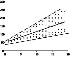
Linear regression needs the relationship between the independent and dependent variables to be linear. It is also important to check for outliers since linear regression is sensitive to outliers effects. The linearity assumption can best be tested with scatter plots, the following two examples depict two cases, where no and little linearity is present.

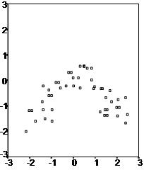
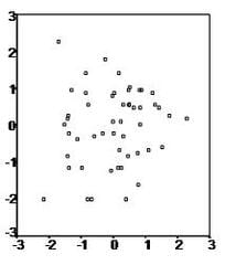
In the cases like these, one should try some non-linear transformations first to make the relationship linear.

NormalitySection titled Normality

The linear regression analysis requires all variables to be multivariate normal. This assumption can best be checked with a histogram or a Q-Q Plot.

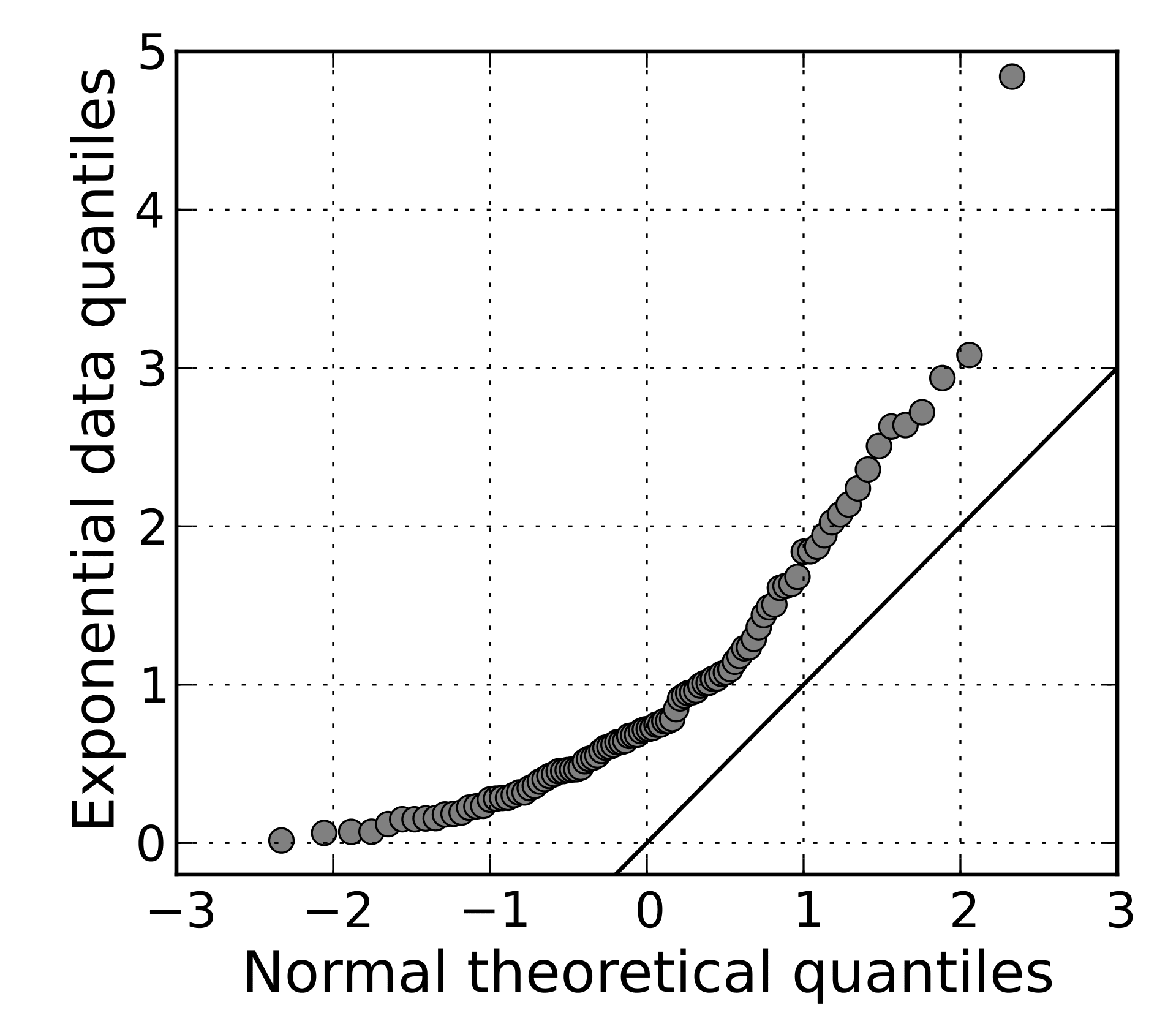
The linear relationship in the first plot shows the normality, however in the second plot, since the data has been picked from an exponential distribution, the Q-Q plot deviates significantly from the linear behavior.

Normality can be also checked with a goodness of fit test, e.g., the Kolmogorov-Smirnov test.

When the data is not normally distributed a non-linear transformation (e.g., log-transformation) might fix this issue.

Lack of perfect multicollinearitySection titled Lack of perfect multicollinearity

Linear regression assumes that there is little or no multicollinearity in the data. Multicollinearity occurs when the independent variables are highly correlated with each other. It can be tested with three primary criteria:

• Correlation matrix – when computing the matrix of Pearson’s Bivariate Correlation among all independent variables the correlation coefficients need to be smaller than 1.

• Tolerance – the tolerance measures the influence of one independent variable on all other independent variables; the tolerance is calculated with an initial linear regression analysis. Tolerance is defined as $T = 1 – R^2$ for these first step regression analysis. With $T < 0.1$ there might be multicollinearity in the data and with $T < 0.01$ there certainly is. Here, $R^2$ is coefficient of determination and is calculated as:

where, $\bar{y}$ is the average response.

• Variance Inflation Factor (VIF) – the variance inflation factor of the linear regression is defined as $VIF = 1/T$. $VIF > 10$ is an indication of presence of multicollinearity; while $VIF > 100$ indicates certainty of presence of multicollinearity. If multicollinearity is found in the data, centering the data (that is deducting the mean of the variable from each score) might help to solve the problem. However, the simplest way to address the problem is to remove independent variables with high VIF values.

A list of more detailed tests can be found at Wikipedia.

No AutocorrelationSection titled No Autocorrelation

Linear regression analysis requires that there is little or no autocorrelation in the data. Autocorrelation occurs when the residuals are not independent from each other. This assumption may be violated in the context of time series data, panel data, cluster samples, hierarchical data, repeated measures data, longitudinal data, and other data with dependencies. In such cases generalized least squares provides a better alternative than the OLS.

While a scatter plot allows you to check for autocorrelations, you can test the linear regression model for autocorrelation with the Durbin-Watson test. Durbin-Watson’s $d$ tests the null hypothesis that the residuals are not linearly auto-correlated. While $d$ can assume values between 0 and 4, values around 2 indicate no autocorrelation. As a rule of thumb, values of $1.5 < d < 2.5$ show that there is no auto-correlation in the data. However, the Durbin-Watson test only analyses linear autocorrelation and only between direct neighbors, which are first order effects.

HomoscedasticitySection titled Homoscedasticity

Homoscedasticity requires that the error term has the same variance $\sigma^2 = \mathbb{E} \big [ \epsilon_i^2 | X]$ in each observation. The scatter plot is good way to check whether the data are homoscedastic (meaning the residuals are equal across the regression line). The following scatter plots show examples of data that are not homoscedastic (i.e., heteroscedastic):

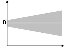
The Goldfeld-Quandt Test can also be used to test for heteroscedasticity. The test splits the data into two groups and tests to see if the variances of the residuals are similar across the groups. If homoscedasticity is present, a non-linear correction might fix the problem.

Key Regression MetricsSection titled Key Regression Metrics

As seen above, residual sum of squares (RSS) is one summary statistics to measure goodness of fir for linear regression models. However, RSS is not the only and most optimal metric that one should study.

Mean Absolute ErrorSection titled Mean Absolute Error

The mean absolute error (MAE) is the simplest regression error metric to understand. In this metric we will calculate the residual for every data point, taking only the absolute value of each so that negative and positive residuals do not cancel out. We then take the average of all these residuals. Effectively, MAE describes the typical magnitude of the residuals.If you are unfamiliar with mean, please have look at my previous post on descriptive statistics.

The MAE is also the most intuitive of the metrics since we’re just looking at the absolute difference between the data and the model’s predictions. Because we use the absolute value of the residual, the MAE does not indicate whether or not the model under or overshoots actual data. Each residual contributes proportionally to the total amount of error, meaning that larger errors will contribute linearly to the overall error. A small MAE suggests the model is great at prediction, while a large MAE suggests that your model may have trouble in certain areas.

Mean Square ErrorSection titled Mean Square Error

Mean square error is the average residual sum of squares:

The effect of the square term in the MSE equation is most apparent with the presence of outliers in our data. While each residual in MAE contributes proportionally to the total error, the error grows quadratically in MSE. This ultimately means that outliers in our data will contribute to much higher total error in the MSE than they would for the MAE. Similarly, our model will be penalized more for making predictions that differ greatly from the corresponding actual value. This is to say that large differences between actual and predicted are punished more in MSE than in MAE.

Root Mean Squared Error (RMSE)Section titled Root Mean Squared Error (RMSE)

As the name suggests, it is the square root of the MSE. Because the MSE is squared, its units do not match that of the original output. It is often used to convert the error metric back into similar units, making interpretation easier. Since the MSE and RMSE both square the residual, they are similarly affected by outliers. The RMSE is analogous to the standard deviation (MSE to variance) and is a measure of how large your residuals are spread out.

Both MAE and MSE can range from 0 to $+ \infty$, so as both of these measures get higher, it becomes harder to interpret how well your model is performing. Another way we can summarize our collection of residuals is by using percentages so that each prediction is scaled against the value it’s supposed to estimate.

Mean absolute percentage error (MAPE)Section titled Mean absolute percentage error (MAPE)

The mean absolute percentage error (MAPE) is the percentage equivalent of MAE. The equation looks just like that of MAE, but with adjustments to convert everything into percentages.

Just as MAE is the average magnitude of error produced by your model, the MAPE is how far the model’s predictions are off from their corresponding outputs on average. Like MAE, MAPE also has a clear interpretation since percentages are easier for people to conceptualize. Both MAPE and MAE are robust to the effects of outliers thanks to the use of absolute value.

However for all of its advantages, we are more limited in using MAPE than we are MAE. MAPE is undefined for data points where the value is 0. Similarly, the MAPE can grow unexpectedly large if the actual values are exceptionally small themselves. Finally, the MAPE is biased towards predictions that are systematically less than the actual values themselves. That is to say, MAPE will be lower when the prediction is lower than the actual compared to a prediction that is higher by the same amount.

Mean Percentage Error (MPE)Section titled Mean Percentage Error (MPE)

The mean percentage error (MPE) equation is exactly like that of MAPE. The only difference is that it lacks the absolute value operation.

Since positive and negative errors will cancel out, we cannot make any statements about how well the model predictions perform overall. However, if there are more negative or positive errors, this bias will show up in the MPE. Unlike MAE and MAPE, MPE is useful to us because it allows us to see if our model systematically underestimates (more negative error) or overestimates (positive error).

In addition to these metrics, you can also take a look at some additional metrics in scikit-learn.

We can also evaluate linear regression models by $R^2$ and Adjusted $R^2$.

R-squaredSection titled R-squared

Also called as coefficient of determination, It determines how much of the total variation in Y (dependent variable) is explained by the variation in X (independent variable). Mathematically, it can be written as:

where, $\bar{y}$ is the average response. The value of R-square is always between 0 and 1, where 0 means that the model does not model explain any variability in the target variable (Y) and 1 meaning it explains full variability in the target variable.

Adjusted R-squaredSection titled Adjusted R-squared

A major drawback of $R^2$ is that if new predictors ($X$) are added to our model, $R^2$ only increases or remains constant but it never decreases. We can not judge that by increasing complexity of our model.

The Adjusted $R^2$ is the modified form of $R^2$ that has been adjusted for the number of predictors in the model. It incorporates model’s degree of freedom. The adjusted $R^2$ only increases if the new term improves the model accuracy.

Here, $N$ is number of samples and $p$ is the number of predictors in the model.

Regularization: Ridge and Lasso RegressionSection titled Regularization: Ridge and Lasso Regression

One of the major aspects of training your machine learning model is avoiding over-fitting. The model will have a low accuracy if it is over-fitting. This happens because your model is trying too hard to capture the noise in your training dataset.

There are various ways to overcome the problem of over-fitting. In terms of linear regression, one of the most common ways is via regularization.

In linear regression, as seen above, the fitting procedure involves a loss function, known as residual sum of squares or RSS. The coefficients, i.e. the weights $\mathbf w$ are chosen, such that they minimize this loss function. Regularization’s’ role is to shrink these learned estimates $\mathbf w$ towards zero.

Two common ways to implement this are:

Ridge Regression

Ridge regression adds the “squared magnitude” of coefficient as penalty term to the loss function.

Here $\lambda$ controls the regularization term, a low value takes us closer to regular regression model.

Lasso Regression

Lasso regression adds the “absolute magnitude” of coefficients as penalty term to the loss function.

The key difference between these techniques is that Lasso shrinks the less important feature’s coefficient to 0 thus, removing some feature altogether. So, this works well for feature selection in case we have a huge number of features.

One of the prime differences between Lasso and Ridge regression is that in ridge regression, as the penalty is increased, all parameters are reduced while still remaining non-zero, while in Lasso, increasing the penalty will cause more and more of the parameters to be driven to zero.

Elastic Net Regression

Elastic net regression is a hybrid algorithm of ridge and lasso regressions. In this case we use both $L1$ and $L2$ terms for regularizing model coefficients:

A Bayesian PerspectiveSection titled A Bayesian Perspective

Although a complete Bayesian perspective of linear regression is complete post in itself, Here I just want to highlight the similarity of ridge and lasso regression techniques with the Bayesian methods. Effectively, when you are using any of these regularization schemes, you are giving a Bayesian treatment to the model.

In the Bayesian framework, the choice of the regularizer is analogous to the choice of prior over the weights. If a Gaussian prior is used, then the Maximum a Posteriori (MAP) solution will be the same as if an L2 penalty was used (Ridge Regression). Whilst not directly equivalent, the Laplace prior (which is sharply peaked around zero, unlike the Gaussian which is smooth around zero), produces the same shrinkage effect to the L1 penalty (Lasso Regression).

You can read about the Bayesian Lasso in more detail here.

Generalization of Linear RegressionSection titled Generalization of Linear Regression

Finally, we will look at some of the generalizations of linear regression. These applications should be able to convince you the wide application of these methods across different fields.

Polynomial RegressionSection titled Polynomial Regression

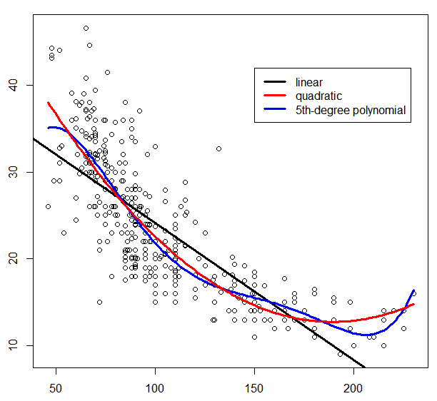
Polynomial regression is a form of regression analysis in which the relationship between the independent variable $x$ and the dependent variable $y$ is modelled as an n-th degree polynomial in $x$. Polynomial regression fits a nonlinear relationship between the value of $x$ and the corresponding conditional mean of $y$.

Mathematically, suppose the N-point data is of form $(x_i, y_i)$ for $1 \leqslant i \leqslant N$. The goal is to find a polynomial approximation of the data by minimizing the residual:

Similar to the OLS problem, this can be viewed as the problem of solving overdetermined system:

This can be solved by the same mathematical tools as the OLS problem. The same set of regression techniques as above can be also applied here. The equation have been used for a polynomial of degree 2, but cam be easily expanded to higher orders. In practice, the choice of order of polynomial is just an additional hyper parameter of the model.

Signal SmoothingSection titled Signal Smoothing

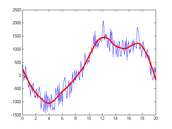
One approach to smooth a noisy signal is based on least squares weighted regularization. The idea is to obtain a signal similar to the noisy one, but smoother. The smoothness of a signal can be measured by the energy of its derivative (or second-order derivative). The smoother a signal is, the smaller the energy of its derivative is.

Let us define a matrix D as,

Then $D\mathbf x$ is the second-order difference (a discrete form of the second-order derivative) of the signal $\mathbf x$. If $\mathbf x$ is smooth, then $\lVert D \mathbf x \rVert^2$ is small in value. Hence, we can propose the signal smoothing as a linear regression problem, where $\mathbf y$ is a noisy signal, that can be smoothened by $\mathbf x$, if we minimize the following loss function:

This can be solved by the same mathematical tools that we used above to solve for ordinary least squares.

Hopefully, this has been able to provide more clarity for linear regression methods. You can use scikit-learn to make linear regression models with your data. Given the simplicity of these API, I have omitted any example from this post. Please let me know in comments below, if you have any suggestions for improving this article.