Support Vector Machines

In this post we will explore a class of machine learning methods called Support Vector Machines also known commonly as SVM.

IntroductionSection titled Introduction

SVM is a supervised machine learning algorithm which can be used for both classification and regression.

In the simplest classification problem, given some data points each belonging to one of the two classes, the goal is to decide which class a new data point will be in. A simple linear solution to this problem can be viewed in a framework where a data point is viewed as a $p$-dimensional vector, and we want to know whether we can separate such points with a ($p-1$)-dimensional hyperplane.

There are many hyperplanes that might classify the data. One reasonable choice as the best hyperplane is the one that represents the largest separation, or margin, between the two classes. So we choose the hyperplane so that the distance from it to the nearest data point on each side is maximized. If such a hyperplane exists, it is known as the maximum-margin hyperplane and the linear classifier it defines is known as a maximum margin classifier; or equivalently, the perceptron of optimal stability.

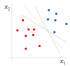
The figure on the right is a binary classification problem (points labeled $y_i = \pm 1$) that is linearly separable in space defined by the vector x. Green and purple line separate two classes with a small margin, whereas yellow line separates them with the maximum margin.

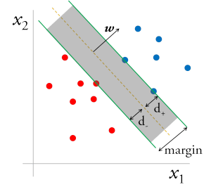
Mathematically, for the linearly separable case, any point x lying on the separating hyperplane satisfies: $\mathbf{x}^T\mathbf{w} + b = 0$, where $\mathbf{w}$ is the vector normal to the hyperplane, and $b$ is a constant that describes how much plane is shifted relative to the origin. The distance of the hyperplane from the origin is $\frac{b}{\lVert \mathbf{w} \rVert}$.

Now draw parallel planes on either side of the decision boundary, so we have what looks like a channel, with the decision boundary as the central line, and the additional planes as gutters. The margin, i.e. the width of the channel, is $(d_+ + d_-)$ and is restricted by the data points closest to the boundary, which lie on the gutters. The two bounding hyperplanes of the channel can be represented by a constant shift in the decision boundary. In other words, these planes ensure that all the points are at least a signed distance d away from the decision boundary. The channel region can be also represented by the following equations:

These conditions can be put more succinctly as:

Using the formulation of distance from origin of three hyper planes, we can show that, the margin, M is equivalent to $d_+ + d_- = \frac{2a}{\lVert \mathbf{w} \rVert}$. Without any loss of generality, we can set $a = 1$, since it only sets the scale (units) of $b$ and $\mathbf{w}$. So to maximize the margin, we have to maximize $1 / \lVert \mathbf{w} \rVert$. Such a non-convex objective function can be avoided if we choose in stead to minimize ${\lVert \mathbf{w} \rVert}^2$.

In summary, for a problem with m numbers of training data points, we need to solve the following quadratic programming problem:

This can be more conveniently put as:

The maximal margin classifier is a very natural way to perform classification, if a separating hyper plane exists. However, in most real-life cases no separating hyper plane exists, and so there is no maximal margin classifier.

Support Vector ClassifierSection titled Support Vector Classifier

We can extend the concept of a separating hyper plane in order to develop a hyper plane that almost separates the classes, using a so-called soft margin. The generalization of the maximal margin classifier to the non-separable case is known as the support vector classifier.

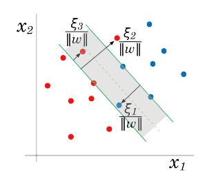
Assuming the classes overlap in the given feature space. One way to deal with the overlap is to still maximize M, but allow for some points to be on the wrong side of the margin. In order to allow these, we can define the slack variables as, $\xi = ( \xi_1, \xi_2 \ldots \xi_m)$. Now, keeping the above optimization problem as a convex problem, we can modify the constraints as:

We can think of this formulation in the following context. The value $\xi_i$ in the constraint $y_i (\mathbf{x}_i^T\mathbf{w} + b) \ge M(1-\xi_i)$ is the proportional amount by which the prediction $f(x_i)=x_i^T\mathbf{w} + b$ is on the wrong side of its margin. Hence by bounding the sum $\sum \xi_i$, we can bound the total proportional amount by which predictions fall on the wrong side of their margin. Mis-classifications occur when $\xi_i > 1$, so bounding $\sum \xi_i$ at a value K say, bounds the total number of training mis-classifications at K.

Similar to the case of maximum margin classifier, we can rewrite the optimization problem more conveniently as,

Now, the question before us is to find a way to solve this optimization problem efficiently.

The problem above is quadratic with linear constraints, hence is a convex optimization problem. We can describe a quadratic programming solution using Lagrange multipliers and then solving using the Wolfe dual problem.

The Lagrange (primal) function for this problem is:

which we can minimize w.r.t. $\mathbf{w}$, b, and $\xi_i$. Setting the respective derivatives to zero, we get,

as well as the positivity constraints, $\alpha_i$, $\mu_i$, $\xi_i \ge 0, \text{ } \forall i$. By substituting these conditions back into the Lagrange primal function, we get the Wolfe dual of the problem as,

which gives a lower bound on the original objective function of the quadratic programming problem for any feasible point. We maximize $L_D$ subject to $0 \le \alpha_i \le C$ and $\sum_{i=1}^{m} \alpha_i y_i = 0$. In addition to above constraints, the Karush-Kuhn-Tucker (KKT) conditions include the following constraints,

for $i = 1 \ldots m$. Together these equations uniquely characterize the solution to the primal and the dual problem.

Let us look at some special properties of the solution. We can see that the solution for $\mathbf{w}$ has the for

with nonzero coefficients $\hat{\alpha}_i$ only for those i for which $y_i (\mathbf{x}_i^T\mathbf{w} + b) - (1 - \xi_i) = 0$. These i observations are called “support vectors” since $\mathbf{w}$ is represented in terms of them alone. Among these support points, some will lie on the edge of the margin $(\hat{\xi}_i = 0)$, and hence characterized by $0 < \hat{\alpha}_i < C$; the remainder $(\hat{\xi}_i > 0)$ have $\hat{\alpha}_i = C$. Any of these margin points can be used to solve for b. Typically, once can use an average value from all of the solutions from the support points.

In this formulation, C is model hyper parameter and can be used as a regularizer to control the capacity and generalization error of the model.

The Kernel TrickSection titled The Kernel Trick

The support vector classifier described so far finds linear boundaries in the input feature space. As with other linear methods, we can make the procedure more flexible by enlarging the feature space using basis expansions such as polynomials or splines. Generally linear boundaries in the enlarged space achieve better training-class separation, and translate to nonlinear boundaries in the original space. Once the basis functions $h_i(x), i=1 \ldots m$ are selected, the procedure remains same as before.

Now recall that in calculating the actual classifier, we needed only support vector points, i.e. we need smaller amount of computation if data has better training-class separation. Furthermore, if one looks closely, we can find an additional trick. The separating plane can be given by the function:

where, $\langle \mathbf{x} \mathbf{y} \rangle$ denotes inner product of vectors $\mathbf{x}$ and $\mathbf{y}$. This shows us that we can rewrite training phase operations completely in terms of inner products!

If we were to replace linear terms with a predefined non-linear operation $h(x)$, the above formulation of the separating plane will simply modify into:

As before, given $\hat{\alpha_i}$, b can be determined by solving $y_i f(\mathbf{x}_i) = 1$ for any (or all) $x_i$ for which $0 < \hat{\alpha}_i < C$. More importantly, this tells us that we do not need to specify the exact nonlinear transformation $h(x)$ at all, rather only the knowledge of the Kernel function $K(x, x') = \langle h(x)h(x') \rangle$ that computes inner products in the transformed space is enough. Note that for the dual problem to be convex quadratic programming problem, $K$ would need to be symmetric positive semi-definite.

The role of the hyper-parameter $C$ is clearer in an enlarged feature space, since perfect separation is often achievable there. A large value of $C$ will discourage any positive $\xi_i$, and lead to an over-fit wiggly boundary in the original feature space; a small value of $C$ will encourage a small value of $\lVert w \rVert$, which in turn causes $f(x)$ and hence the boundary to be smoother, potentially at the cost of more points as support vectors.

Curse of Dimensionality… huhSection titled Curse of Dimensionality… huh

With m training examples, $p$ predictors and M support vectors, the SVM requires $M^3 + Mm + mpM$ operations. This suggests the choice of the kernel and hence number of support vectors M will play a big role in feasibility of this method. For a really good choice of kernel that leads to very high training-class separation, i.e. $M <<< m$, the method can be viewed as linear in m. However, for a bad choice case, $M \approx m$ we will be looking at an $O (m^3)$ algorithm.

The modern incarnation of deep learning was designed to overcome these limitations (large order of computations and clever problem-specific choice of kernels) of kernel machines. We will look at the details of a generic deep learning algorithm in a future post.