In the previous post on Support Vector Machines (SVM), we looked at the mathematical details of the algorithm. In this post, I will be discussing the practical implementations of SVM for classification as well as regression.
I will be using the iris dataset as an example for the classification problem, and a randomly generated data as an example for the regression problem. In Python, scikit-learn is a widely used library for implementing machine learning algorithms, SVM is also available in scikit-learn library and follow the usual structure (Import library, object creation, fitting model and prediction). The sklearn.svm module provides mainly two classes: sklearn.svm.svc for classification and sklearn.svm.svr for regression.
Table of ContentsSection titled Table of Contents
Open Table of Contents
Preparing Data for SVM ModelsSection titled Preparing Data for SVM Models
As pointed out by Admiral deblue in the comments below, all practical implementations of SVMs have strict requirements for training and testing (prediction). The first requirement is that all data should be numerical. Therefore, if you have categorical features, they need to be converted to numerical values using variable transformation techniques like one-hot-encoding, label-encoding etc. SVM model implementations in python also do not support missing values, hence you need to either remove data with missing values or use some form of data imputing. The sklearn.preprocessing.Imputer module can be quite helpful for this exercise. Furthermore, since SVMs assume that the data it works with is in a standard range, usually either 0 to 1, or -1 to 1 etc. (so that all feature variables are treated equally), it would be best served to use the feature “normalization” before training the model. The sklearn.preprocessing.StandardScaler module can use used for such normalization.
In general, sklearn models require training data (X) to be numpy nd-array and dependent variable (y) as numpy 1-d array. With newer versions of Pandas, Pandas data-frame and series can also be used for providing X and y to sklearn models.
sklearn.pipeline provides an impressive set of tools to deal with various aspects of data preparation for training different models in a coherent manner. This will be a topic of discussion for a post in near future.
SVM for Classification ProblemsSection titled SVM for Classification Problems
The iris dataset is a simple dataset of contains 3 classes of 50 instances each, where each class refers to a type of iris plant. One class is linearly separable from the other two; the latter are NOT linearly separable from each other. Each instance has 4 features:
- sepal length
- sepal width
- petal length
- petal width
A typical problem to solve is to predict the class of the iris plant based on these 4 features. For brevity and visualization, in this example we will be using only the first two features.
Setup for SVM ClassificationSection titled Setup for SVM Classification
Below is the simplest implementation of a SVM for this problem. In this example, we see the simplest implementation of SVM classifier with the linear and the radial basis function (rbf) kernels.
import pandas as pd
import numpy as np
from sklearn import svm, datasets
import matplotlib.pyplot as plt
%matplotlib inline

iris = datasets.load_iris()
X = iris.data[:, :2] # we only take the first two features.
y = iris.target

# Plot resulting Support Vector boundaries with original data
# Create fake input data for prediction that we will use for plotting
# create a mesh to plot in
x_min, x_max = X[:, 0].min() - 1, X[:, 0].max() + 1
y_min, y_max = X[:, 1].min() - 1, X[:, 1].max() + 1
h = (x_max / x_min)/100
xx, yy = np.meshgrid(np.arange(x_min, x_max, h),
np.arange(y_min, y_max, h))
X_plot = np.c_[xx.ravel(), yy.ravel()]

# Create the SVC model object
C = 1.0 # SVM regularization parameter
svc = svm.SVC(kernel='linear', C=C, decision_function_shape='ovr').fit(X, y)
Z = svc.predict(X_plot)
Z = Z.reshape(xx.shape)

plt.figure(figsize=(15, 5))
plt.subplot(121)
plt.contourf(xx, yy, Z, cmap=plt.cm.tab10, alpha=0.3)
plt.scatter(X[:, 0], X[:, 1], c=y, cmap=plt.cm.Set1)
plt.xlabel('Sepal length')
plt.ylabel('Sepal width')
plt.xlim(xx.min(), xx.max())
plt.title('SVC with linear kernel')

# Create the SVC model object
C = 1.0 # SVM regularization parameter
svc = svm.SVC(kernel='rbf', C=C, decision_function_shape='ovr').fit(X, y)

Z = svc.predict(X_plot)
Z = Z.reshape(xx.shape)

plt.subplot(122)
plt.contourf(xx, yy, Z, cmap=plt.cm.tab10, alpha=0.3)
plt.scatter(X[:, 0], X[:, 1], c=y, cmap=plt.cm.Set1)
plt.xlabel('Sepal length')
plt.ylabel('Sepal width')
plt.xlim(xx.min(), xx.max())
plt.title('SVC with RBF kernel')

plt.show()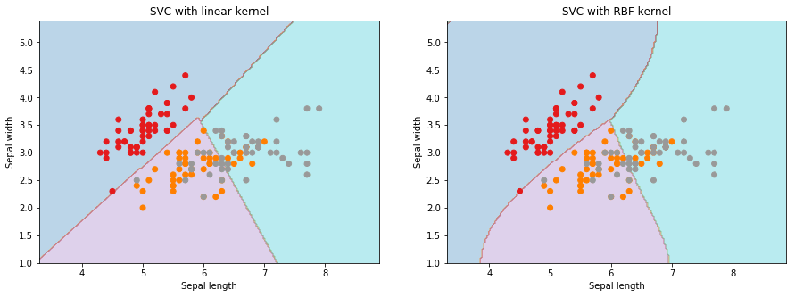
Parameter Tuning for SVM ClassificationSection titled Parameter Tuning for SVM Classification
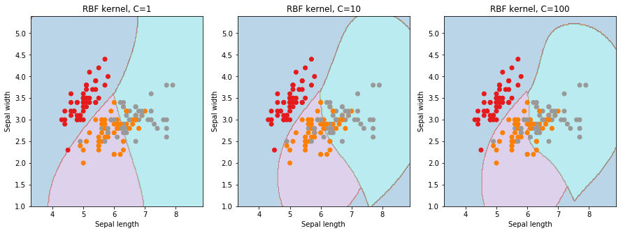
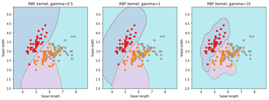
Similar to any machine learning algorithm, we need to choose/tune hyper-parameters for these models. The important parameters to tune are: C (the penalty parameter or the error term. Remember from our last post, this acts as a regularization parameter for SVM) and (Kernel coefficient for ‘rbf’, ‘poly’ and ‘sigmoid’ kernels). In above example, we used a default value of .
Multi-class ClassificationSection titled Multi-class Classification
SVM by definition is well suited for binary classification. In order to perform multi-class classification, the problem needs to be transformed into a set of binary classification problems.
There are two approaches to do this:
One vs. Rest Approach (OvR): This strategy involves training a single classifier per class, with the samples of that class as positive samples and all other samples as negatives. This strategy requires the base classifiers to produce a real-valued confidence score for its decision, rather than just a class label; discrete class labels alone can lead to ambiguities, where multiple classes are predicted for a single sample.
One vs. One Approach (OvO): In the one-vs.-one (OvO) strategy, one trains K(K − 1)/2 binary classifiers for a K-way multi-class problem; each receives the samples of a pair of classes from the original training set, and must learn to distinguish these two classes. At prediction time, a voting scheme is applied: all K(K − 1)/2 classifiers are applied to an unseen sample and the class that got the highest number of “+1” predictions gets predicted by the combined classifier. Like OvR, OvO suffers from ambiguities in that some regions of its input space may receive the same number of votes.
In svm.svc implementation, decision_function_shape parameter provides the option to choose one of
two strategy. Although, by default OvO strategy is chosen for historical reasons, it is always
recommended to switch to the OvR approach.
Let us first understand what effects and parameters have on SVM models. As seen below, we find that higher the value of , it will try to exact fit the as per training data set i.e. generalization error and cause over-fitting problem. controls the trade off between smooth decision boundary and classifying the training points correctly.
We will be using 5-fold cross validation to perform grid search to calculate optimal hyper-parameters. This is easily achieved in scikit-learn using the sklearn.model_selection.GridSearchCV class.
from sklearn.model_selection import train_test_split
from sklearn.model_selection import GridSearchCV
from sklearn.metrics import classification_report
from sklearn.utils import shuffle

# shuffle the dataset
X, y = shuffle(X, y, random_state=0)

# Split the dataset in two equal parts
X_train, X_test, y_train, y_test = train_test_split(
    X, y, test_size=0.25, random_state=0)

# Set the parameters by cross-validation
parameters = [{'kernel': ['rbf'],
               'gamma': [1e-4, 1e-3, 0.01, 0.1, 0.2, 0.5],
                'C': [1, 10, 100, 1000]},
              {'kernel': ['linear'], 'C': [1, 10, 100, 1000]}]

print("# Tuning hyper-parameters")
print()

clf = GridSearchCV(svm.SVC(decision_function_shape='ovr'), parameters, cv=5)
clf.fit(X_train, y_train)

print("Best parameters set found on development set:")
print()
print(clf.best_params_)
print()
print("Grid scores on training set:")
print()
means = clf.cv_results_['mean_test_score']
stds = clf.cv_results_['std_test_score']
for mean, std, params in zip(means, stds, clf.cv_results_['params']):
    print("%0.3f (+/-%0.03f) for %r"
          % (mean, std * 2, params))
print()Output:
# Tuning hyper-parameters

Best parameters set found on development set:

{'C': 1, 'gamma': 0.1, 'kernel': 'rbf'}

Grid scores on training set:

0.634 (+/-0.066) for {'C': 1, 'gamma': 0.0001, 'kernel': 'rbf'}
0.634 (+/-0.066) for {'C': 1, 'gamma': 0.001, 'kernel': 'rbf'}
0.634 (+/-0.066) for {'C': 1, 'gamma': 0.01, 'kernel': 'rbf'}
0.768 (+/-0.168) for {'C': 1, 'gamma': 0.1, 'kernel': 'rbf'}
0.768 (+/-0.161) for {'C': 1, 'gamma': 0.2, 'kernel': 'rbf'}
0.768 (+/-0.173) for {'C': 1, 'gamma': 0.5, 'kernel': 'rbf'}
0.634 (+/-0.066) for {'C': 10, 'gamma': 0.0001, 'kernel': 'rbf'}
0.634 (+/-0.066) for {'C': 10, 'gamma': 0.001, 'kernel': 'rbf'}
0.768 (+/-0.168) for {'C': 10, 'gamma': 0.01, 'kernel': 'rbf'}
0.750 (+/-0.193) for {'C': 10, 'gamma': 0.1, 'kernel': 'rbf'}
0.750 (+/-0.193) for {'C': 10, 'gamma': 0.2, 'kernel': 'rbf'}
0.732 (+/-0.183) for {'C': 10, 'gamma': 0.5, 'kernel': 'rbf'}
0.634 (+/-0.066) for {'C': 100, 'gamma': 0.0001, 'kernel': 'rbf'}
0.768 (+/-0.168) for {'C': 100, 'gamma': 0.001, 'kernel': 'rbf'}
0.759 (+/-0.178) for {'C': 100, 'gamma': 0.01, 'kernel': 'rbf'}
0.741 (+/-0.164) for {'C': 100, 'gamma': 0.1, 'kernel': 'rbf'}
0.723 (+/-0.175) for {'C': 100, 'gamma': 0.2, 'kernel': 'rbf'}
0.732 (+/-0.183) for {'C': 100, 'gamma': 0.5, 'kernel': 'rbf'}
0.768 (+/-0.168) for {'C': 1000, 'gamma': 0.0001, 'kernel': 'rbf'}
0.759 (+/-0.178) for {'C': 1000, 'gamma': 0.001, 'kernel': 'rbf'}
0.750 (+/-0.193) for {'C': 1000, 'gamma': 0.01, 'kernel': 'rbf'}
0.732 (+/-0.183) for {'C': 1000, 'gamma': 0.1, 'kernel': 'rbf'}
0.732 (+/-0.183) for {'C': 1000, 'gamma': 0.2, 'kernel': 'rbf'}
0.696 (+/-0.164) for {'C': 1000, 'gamma': 0.5, 'kernel': 'rbf'}
0.768 (+/-0.173) for {'C': 1, 'kernel': 'linear'}
0.759 (+/-0.178) for {'C': 10, 'kernel': 'linear'}
0.759 (+/-0.178) for {'C': 100, 'kernel': 'linear'}
0.759 (+/-0.178) for {'C': 1000, 'kernel': 'linear'}We have done a few things in above code. Let us break down these in steps.
First, if you pay attention to the input dataset, it lists three different class of iris plants in order. In order for models to be forgetful about such an order, its safer to first shuffle the dataset. This is achieved using the shuffle() method. We also want to take aside a fraction of dataset for final testing of our algorithms success. This is done using the train_test_split() method. In this particular case, we have kept aside about 1/4 th of the dataset for testing.
Moving to the main part of the code: tuning of hyper-parameters for SVM. It is done using the
GridSearchCV() class (The highlighted lines in the above code blocks). At the end, we are also
printing out the accuracy score for different set of parameters. We can find the best set of
parameters by the clf.best_params_ property.
By default scikit-learn uses accuracy as score for classification tasks.
GridSearchCV() provides option to use alternative scoring metrics via the
scoring parameter. Some common alternatives are, precision, recall, auc with
different averaging strategies like micro, macro, weighted etc.
Finally, we can test our model on the test dataset and evaluate various classification metrics
using the classification_report() method.
print("Detailed classification report:")
print()
print("The model is trained on the full development set.")
print("The scores are computed on the full evaluation set.")
print()
y_true, y_pred = y_test, clf.predict(X_test)
print(classification_report(y_true, y_pred))
print()Output:
The model is trained on the full development set. The scores are computed on the full evaluation set.
| id | precision | recall | f1-score | support |
|---|---|---|---|---|
| 0 | 1.00 | 1.00 | 1.00 | 12 |
| 1 | 0.73 | 0.92 | 0.81 | 12 |
| 2 | 0.91 | 0.71 | 0.80 | 14 |
| avg / total | 0.88 | 0.87 | 0.87 | 38 |
Apart from accuracy, three major metrics to understand the task for classification are: precision, recall and f1-score.
Precision: The precision is the ratio tp / (tp + fp) where tp is the number of true
positives and fp the number of false positives. The precision is intuitively the ability of the
classifier not to label as positive a sample that is negative.
Recall: The recall is the ratio tp / (tp + fn) where tp is the number of true positives and
fn the number of false negatives. The recall is intuitively the ability of the classifier to find
all the positive samples.
F1-Score: It can be interpreted as a weighted harmonic mean of the precision and recall, where an f1-score reaches its best value at 1 and worst score at 0.
Support: Although not a scoring metric, it is an important quantity when looking at different
metrics. It is the number of occurrences of each class in y_true.
SVM for Regression ProblemsSection titled SVM for Regression Problems
Let us first generate a random dataset where we want to generate a regression model. In order to
have a good visualization of our results, it would be best to use a single feature as an example.
In order to study effect of non-linear models, we will be generating our data from the sin()
function.
X = np.sort(5 * np.random.rand(200, 1), axis=0)
y = np.sin(X).ravel()
y[::5] += 3 * (0.5 - np.random.rand(40))Setup for SVM RegressionSection titled Setup for SVM Regression
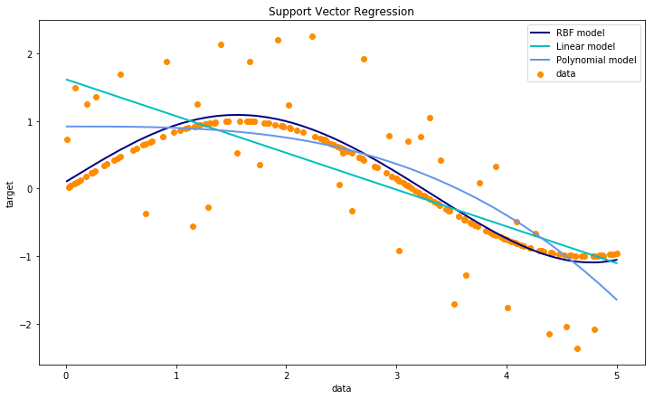
Below is the simplest implementation of a SVM for this regression problem. In sci-kit learn SVM regression models are implemented using the svm.SVR class.
In this example, we see the simplest implementation of SVM regressors with the linear, polynomial of degree 3 and the radial basis function (rbf) kernels.
from sklearn.svm import SVR
svr_rbf = SVR(kernel='rbf', C=1e3, gamma=0.1)
svr_lin = SVR(kernel='linear', C=1e3)
svr_poly = SVR(kernel='poly', C=1e3, degree=3)
y_rbf = svr_rbf.fit(X, y).predict(X)
y_lin = svr_lin.fit(X, y).predict(X)
y_poly = svr_poly.fit(X, y).predict(X)

lw = 2
plt.figure(figsize=(12, 7))
plt.scatter(X, y, color='darkorange', label='data')
plt.plot(X, y_rbf, color='navy', lw=lw, label='RBF model')
plt.plot(X, y_lin, color='c', lw=lw, label='Linear model')
plt.plot(X, y_poly, color='cornflowerblue', lw=lw, label='Polynomial model')
plt.xlabel('data')
plt.ylabel('target')
plt.title('Support Vector Regression')
plt.legend()
plt.show()Output:
Parameter Tuning for SVM RegressionSection titled Parameter Tuning for SVM Regression
The common hyper-parameters in the case of SVM regressors are: (the error term),
(specifies the epsilon-tube within which no penalty is associated in the training loss function
with points predicted within a distance epsilon from the actual value) and (Kernel
coefficient for ‘rbf’, ‘poly’ and ‘sigmoid’ kernels). Given our example is extremely simplified, we
won’t be able to observe any significant impact of any of these parameters. In general, similar to
classification case, GridSearchCV can be used to tune SVM regression models as well.
ConclusionsSection titled Conclusions
So that brings us to an end to the different aspects of Support Vector Machine algorithms. In the first post on the topic, I described the theory and the mathematical formulation of the algorithm. In this post, I discussed the implementation details in Python and ways to tune various hyper-parameters in both classification and regression cases. From practical experience, SVMs are great for:
- Small to medium data sets only. Training becomes extremely slow in the case of larger datasets.
- Data sets with low noise. When the data set has more noise i.e. target classes are overlapping, SVM perform very poorly.
- When feature dimensions are very large. SVMs are extremely helpful specially when no. of features is larger than no. of samples.
- Since only a subset of training points are used in the decision function (called support vectors), it is quite memory efficient. This also leads to extremely fast prediction.
An important point to note is that the SVM doesn’t directly provide probability estimates, these are calculated using an expensive cross-validation in scikit-learn implementation.
Finally, as would be the case with any machine learning algorithm, I would suggest you to use SVM and analyze the power of SVMs by tuning various hyper-parameters. I want to hear your experience with SVM, how have you tuned SVM models to avoid over-fitting and reduce the training time? Please share your views and experiences in the comments below.
COMMENTS